

Seal Abundance and Distribution
Background
Atlantic grey seals and harbour seals reside across the North-East Atlantic Ocean. As top predators, seals can be used as an indicator to reflect the state of the marine ecosystem. This assessment of seal abundance and distribution aims to determine if populations of both species are in a healthy state, with no long-term decrease in population size, beyond natural variability. Historically, populations have declined due to anthropogenic influences. This assessment will help to determine trends in abundance.
Seal abundance and distribution are influenced by many factors, such as disease, pollutants, competition with other species, changes in the distribution and abundance of prey, disturbance, and anthropogenic removals such as by-catch, hunting and culling. Seals were hunted well into the 20th century, resulting in depleted populations across OSPAR Regions. Protective legislation to reduce those anthropogenic threats has supported the recovery of colonies in more recent years, however the legal removal of seals to protect fisheries or for hunts is still carried out and the threat from by-catch remains present across many areas.
Changes in distribution or declines in abundance identified as part of the assessment may signal that seals within Assessment Units (AUs) are not in a healthy state. Further investigations into identifying the cause (natural or human-induced), assessing the relationship between such pressures and outcomes, may then be required to determine appropriate management measures.
The conservation status of harbour seals and grey seals is also assessed under the European Union Habitats Directive (Council Directive 92/43/EEC).
 © Julia Sutherland")
Figure 1: Harbour seals (Phoca vitulina) © Julia Sutherland
 © Niki Clear, JNCC")
Figure 2: Atlantic grey seals (Halichoerus grypus) © Niki Clear, JNCC
Grey and harbour seal populations are widespread across the North-East Atlantic Ocean. Both species forage in coastal and open sea, however they return to land-based haul-out sites where they rest, moult and breed. These haul-out sites may be utilised by individual seals either on a year-round basis or at specific times of year for either breeding or moulting. While harbour seals commonly forage within 50 km of their chosen haul-out site, grey seals often forage at more offshore sites (over 100 km from land) and may utilise many different haul-out sites during the year.
Seal population status was highlighted in the OSPAR Quality Status Report (QSR) 2010 by means of the two OSPAR Ecological Quality Objectives (EcoQOs) applied in the Greater North Sea (Region II) which assessed pup production in grey seals and population size in harbour seals. The harbour seal EcoQO was not met in several areas, where declines in local seal populations of more than 10% occurred between 2001 and 2006 (Shetland, Orkney, east of Scotland, Greater Wash to Scroby Sands, Limfjorden in Denmark, and the west coast of Norway). Both the east of England and Limfjorden had been affected by phocine distemper virus (PDV) in the years assessed. The reasons for changes in the other areas were not yet clear. The EcoQO for no decline of greater than 10% in grey seal pup production over a five-year running mean was assessed as met in all areas of Region II within relevant sub-units where data were reported. It should be noted that the North Sea EcoQOs are not equivalent to either of the threshold values applied in this assessment.
Results from the OSPAR Intermediate Assessment (IA) 2017 , where new Assessment Units (AUs) were delineated for both species, demonstrated that harbour seal abundance was stable or increasing across most of the Region II but was declining in some Scottish AUs. In contrast, grey seal abundance was increasing, and distribution was stable across the combined Region II and UK parts of Region III assessment unit. The reasons for harbour seal declines in some units and stabilisation in others were unclear and triggered the commencement of further investigation for the early detection of similar trends elsewhere.
The QSR 2023 expands upon those OSPAR Regions assessed within the IA2017, now encompassing Region II, the whole of Region III, out to the Marine Strategy Framework Directive (MSFD) boundary and the addition of Region I. The expansion into the Arctic Waters (Region I) will allow for more latitudinal variation in the examination of indicator trends, particularly concerning the effects of environmental change. The expansion is in line with the OSPAR NEAES 2030 S5.O4: By 2025 at the latest OSPAR will take appropriate actions to prevent or reduce pressures to enable the recovery of marine species and benthic and pelagic habitats in order to reach and maintain good environmental status as reflected in relevant OSPAR status assessments, with action by 2023 to halt the decline of marine birds.
When linked and compared with suitable pressure indicators, assessments of abundance trends within and across OSPAR Regions can provide key insights into the drivers of observed changes and help inform appropriate management of those pressures, especially where individuals may move between AUs and wider regions.
Grey seal and harbour seal were also assessed under the Habitat Directive Article 17 reporting in 2019 (EU, 2019).
Overview
This indicator assessment uses estimates of seal numbers from monitoring programmes that count seals on land when they are moulting or breeding, for two species: Atlantic grey seal (Halichoerus grypus) and harbour seal (Phoca vitulina).
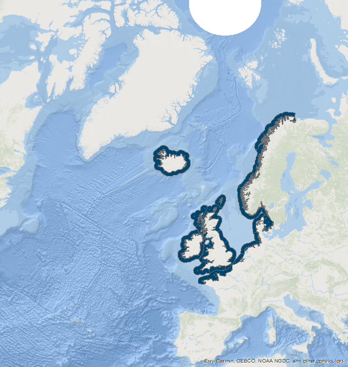
Assessments of changes in abundance and distribution were made within discrete geographical areas of coastline, or ‘Assessment Units’ (AUs). The large number of small AUs for harbour seals (Figure a) reflects a balance between population structure evidence (e.g. telemetry and genetics) and feasible monitoring sites (Carroll et al., 2020). Similar research methods demonstrated that grey seals commonly forage across much wider areas, and visit numerous different sites over a year, so their abundance is assessed across the whole of OSPAR Regions I, II and III using a single AU (Figure b).
Seal abundance surveys are not designed to detect changes in distribution; they can only reflect the distribution of seals at specific times of the year (moult or breeding seasons). Therefore, change in distribution within AUs is used as a ‘surveillance indicator’ to help interpret changes in abundance. Given the scale of the distribution data provided for grey seals, the same coastal based AUs used for harbour seal abundance and distribution are also used to evaluate grey seal distribution in this indicator. The distribution metrics are not compared to any formal threshold values.
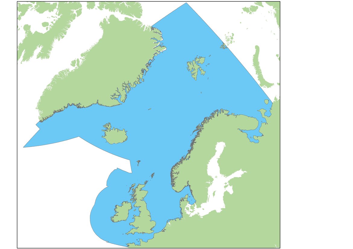
Figure b: Assessment Unit (in blue) for grey seal abundance.
Available at: ODIMS
 for harbour seal abundance and distribution of harbour seal and grey seal.")
Figure a: Assessment Units (AUs) for harbour seal abundance and distribution of harbour seal and grey seal.
Key: 1. South-West Scotland, 2. West Scotland, 3. Western Isles, 4. North coast & Orkney, 5. Shetland, 6. Moray Firth, 7. East Scotland, 8. North-East England, 9. South-East England, 10. South England, 11. South-West England, 12. Wales, 13. North-West England, 14. Northern Ireland, 15. Ireland, 16. French North Sea & Channel coast, 17. Belgium coast and Dutch Delta, 18. Wadden Sea, 19. Limfjorden, 20. Kattegat, 21. Iceland, 22. Skagerrak, 23. Norway (Hvaler – Stad), 24. Norway (Stad – Vesterålen), 25. Norway (Troms – Finnmark)
[Grey seal abundance has been assessed at a larger scale with a single AU covering OSPAR Regions I, II and III, but for the purpose of analysis, data was requested at the scale of the units presented in this figure.]
Available at: ODIMS
Seal Monitoring in the North-East Atlantic
Grey seals and harbour seals are surveyed when they come ashore (‘haul-out’) and can be most easily counted. Survey coverage and monitoring effort of both species is commonly higher where they are most abundant. In some AUs, monitoring is undertaken in specific areas by local organisations and does not form part of synoptic national survey programmes. Surveys are usually conducted from the air but may also be conducted from land or by boat. In most areas, aerial surveyors take photographs of the haul-out sites and animals are later counted from the images (see example in Figure c).
")
Figure c: Mixed species colony of seals hauled-out during a UK aerial monitoring survey (courtesy of Callan Duck, Sea Mammal Research Unit)
There are two periods during the year when most grey and harbour seal surveys take place: breeding (pupping) and moulting. Harbour seals give birth to pups in early summer and moult after breeding in late summer. Atlantic grey seals pup in the autumn or winter and moult in early spring. The frequency of surveys during these periods varies across OSPAR Contracting Parties due to differences in the total number of resident animals, funding, geography, and historical development of the monitoring programmes. Repeated surveys of both grey and harbour seals throughout the year are not economically feasible and Contracting Parties use population censuses in one or perhaps two seasons of the year. Particularly for grey seals, it is challenging to select an ideal single time to survey as there is the potential for differences between the breeding population and the population that is present during other times of the year (Russell et al., 2013; Brasseur et al., 2015).
All Contracting Parties have some form of monitoring in place for harbour seals during their annual summer moulting period. This is when the probability that animals will haul-out and be detectable during a survey is highest and provides an index for calculation of an abundance estimate or trend. Telemetry data are also used to estimate the proportion of seals that are hauled-out, and available to be counted during the survey window. In some Contracting Parties, harbour seal pup numbers are also recorded, however these data are not included as part of OSPAR assessments.
Grey seals are often counted alongside harbour seals during these moult surveys by several Contracting Parties, though the number of grey seals hauled-out during the harbour seal moult can be very variable from year to year. Within Germany, the Netherlands and Denmark, monitoring of this nature covers the Wadden Sea area only and is carried out under the Trilateral Monitoring and Assessment Programme (TMAP), coordinated by the Trilateral Seal Expert Group (EG-Seals).
Survey coverage and monitoring effort of both species is commonly higher where they are most abundant. In some AUs monitoring is undertaken in specific areas by local organisations and does not form part of synoptic national survey programmes. Annex 2 and 3 within the M3 CEMP (Coordinated Environmental Monitoring Programme) Guideline provides details of grey and harbour seal monitoring programmes in each AU.
Data Collation
Following a data call in February 2021, all Contracting Parties were asked to provide data on grey seals and harbour seals for the period 1992–2019. Data for both species were received from the UK, Ireland, France, Belgium, Germany, the Netherlands, Denmark, Sweden, Norway, Iceland, and Greenland.
Given the scale of coastal monitoring for grey seals, data were requested to be provided at the same scale of coastal AUs used for harbour seal abundance and distribution (hereby referred to as sub-AUs when associated with assessments of grey seal abundance). Counts were requested for individual haul-out sites (both species) and breeding colonies (grey seals only). For the most part, counts provided on the AU/sub-AU level and used for abundance trend analyses and fine-scale individual haul-out and/or colony site data were used for the distribution analyses.
For Limfjorden and Kattegat sub-AUs (AUs 19 and 20), grey seal monitoring data were provided on the haul-out level, but not at the sub-AU scale. The frequency and spatial distribution of the data precluded its aggregation to the sub-AU level. Thus, these relevant sub-AUs were not able to be considered for abundance analysis but were considered as part of the evaluation of grey seal distribution. Harbour seal data for these AUs were provided on both a fine and AU scale and thus were considered for both the abundance assessment and distribution indicator.
Data submissions from Norway were supplemented by descriptive evidence summaries to support the indicator. Belgium noted limited seal presence and suitable data and so provided descriptive evidence to support the overall AU assessment.
Iceland estimates grey seal population size using pup count data collected during the breeding season in autumn, meaning that population estimates were not comparable with data provided by other Contracting Parties. During harbour seal monitoring surveys in summer, if grey seals were also sighted, these were recorded (Granquist, 2021). It was not however possible to acquire this data in time for the data call and so a qualitative summary of grey seal abundance trends has been included for this indicator.
Greenland noted that not enough annual counts have thus far been conducted in the country, and that harbour and grey seal presence is infrequent and limited. Similarly, for the Faroe Isles, only grey seals breed there and counts only commenced in 2018. Therefore, assessments were not able to be generated for these countries and instead, descriptive data have been provided to supply an overview of seal presence within these waters. Countries within the Bay of Biscay and Iberian Coast (Region IV) (France, Spain and Portugal) have also provided anecdotal evidence of intermittent grey seal presence on their coasts. It is thought that these seals may be travelling from those resident French colonies within Region III.
Although numbers from these noted countries are considered as marginal compared to those larger, frequently monitored haul-out sites and colonies in neighbouring countries, they are recorded in an OSPAR framework for completeness.
Subsets
It is not always possible to survey the entire extent of an AU within a monitoring cycle due to either financial or time constraints. Thus, seal haul-out and breeding sites may also not always have been monitored at the scale of the AUs.
On occasion, a more comprehensive time series of data was available from a subset of the AU than at the whole AU level. For example, for many UK AUs, subsets of more frequently monitored data were employed for grey and harbour seal abundance assessments. For these AUs the subset was used as a proxy to allow robust trend fitting.
Upon receiving data via the data call, AU totals from France did not match the totals from the fine scale data, and thus totals were generated on an AU and subset scale from the fine scale data by the contracted data analysts. For the Belgium coast & Dutch Delta (AU 17) totals, annual surveys within the fourth survey polygon (Grevelingen) commenced only in 2010 due to previous low occupancy. Thus, a time series of a subset was generated using the fine scale data from the remaining three survey polygons within the Dutch Delta. The occupancy of harbour seals within the Grevelingen region is noted as part of outputs for this AU. Following a minor amendment to the AU 20 boundary after the data call, additional data for the Kattegat (AU 20) comprising updated counts was also included.
The confidence in the trends generated using these subsets is much increased when compared to those produced by the AU level data alone given the higher number of data points available for the models and can provide an indication of trends for the wider AU. Where subsets have been utilised, the percentage coverage of the subset when compared to the whole AU has been provided (Table c).
Assessing Trends in Grey Seal Abundance
The UK and Ireland do not usually collect grey seal data during their moult, and so no moult count data were available to be analysed for these AUs (AUs 1-15). Data provided and used in this assessment comprised: grey seal counts conducted during surveys of harbour seals in their summer moult period (August) (UK and Ireland) and counts during the grey seal moult period which follows the breeding season in early spring, depending on the Contracting Party (continental Europe).
To describe changes of abundance of grey seals for the indicator, counts of grey seals at haul-outs during August or moult surveys (depending on the Contracting Party) were analysed and trends fitted (where possible) on a ‘sub-Assessment Unit’ scale and combined for an assessment across the OSPAR Assessment Unit. However, spatial variation in survey effort, protocol (summer vs moult counts) and difference in the number of animals available to count* meant that counts could not be combined across the single AU. Instead, trends were fitted to counts of grey seals at the scale of those AUs utilised for seal distribution and harbour seal abundance before being combined for an assessment across the single AU. This has resulted in two predicted trends in abundance for grey seals as part of this indicator (M3): (1) UK and Ireland and (2) continental Europe.
*Summer and moult counts represent very different proportions of the population; approximately 25% of grey seals are hauled out during the survey windows in August (Russell & Carter 2021; SCOS 2021) whereas a much higher proportion is hauled-out during the moult.
Assessing Trends in Harbour Seal Abundance
Harbour seal abundance is assessed using counts of harbour seals on land at haul-out sites during moult as an index of abundance within each assessment unit. This proxy for population size is an underestimate of the true population size as it includes only those animals hauled-out at the time of counting. This metric was previously used to construct the EcoQO on harbour seals.
For example, 72% (95% CI: 54–88) of the population in Scotland are estimated to be hauled out during the summer moult survey window (Lonergan et al. 2013). The type of counts provided by Contracting Parties varied (single counts, maximum or mean counts) but were consistent within AU. AU totals provided by the Contracting Parties were used directly in the analysis with those exceptions detailed in (Subsets).
Harbour Seal and Grey Seal Threshold Values and Baselines
Two threshold values were used to assess grey and harbour seal abundance in each AU in relation to baselines described below. The use of the two threshold values aims to provide an indicator that would warn against both a slow but long-term steady decline and against a recovery followed by a subsequent decline (potentially missed with a fixed baseline set below reference conditions). The two threshold values together would be able to act as a trigger for investigation of any necessary management measures to promote recovery.
Threshold Value 1:
- No decline in seal abundance of >1% per year in the previous six-year period (this is approximately 6% over 6 years).
This uses a rolling baseline (Method 1; OSPAR, 2012) based on the most recent six-year period, seeking to identify if seal populations are maintained, with no decrease in population size with regard to the (short-term) baseline (beyond natural variability (<1% per year)) and to identify if efforts are needed to restore populations, where they have deteriorated due to anthropogenic influences, to a healthy state.
To estimate the annual increase or decrease in the number of animals counted within the most recent six-year reporting round, the fitted trend abundance in 2014 was compared against that of 2019.
To avoid the problem of shifting baselines (see M3 CEMP Guidelines) when using the rolling baseline applied in Threshold Value 1, a threshold value relating to a fixed, historic baseline is also needed (Threshold Value 2).
Threshold Value 2:
- No decline in seal abundance of >25% since the fixed baseline in 1992 (or closest value).
The baseline chosen (1992) relates to that used by some Member States for reporting under the European Union Habitats Directive (Council Directive 92/43/EEC) (or if such data are not available, the start of the data series). Testing shows that there is sufficient monitoring to assess against this threshold value with confidence. It should however be noted that if data are not available from 1992, and a shorter timescale is assessed, the 25% decline since the baseline is not equivalent to those AUs where data do extend to 1992 (i.e. a 25% decline since 2003 would describe a more rapid contraction in the population than a 25% decline since 1992).
To estimate the annual increase or decrease in the number of animals counted within the long-term time period, the fitted trend abundance in 1992* was compared against that of 2019.
*Data as far back as 1992 were not available in all AUs; in such cases, the closest year following 1992 was used as a historical baseline. Indicator threshold values were set as a deviation from the baseline value (Method 3; OSPAR, 2012).
Appropriateness of Historic Baseline (1992)
The fixed 1992 (historical) baseline reflects a point in time when populations were already subject to anthropogenic pressures including culling or natural pressures such as PDV outbreaks (in harbour seals), so this baseline year most likely represents a time when populations had not yet recovered from severe depletion.
Seals have been historically hunted both illegally and legally and it is not possible to know the undisturbed state, nor, for some areas, the current carrying capacity that could be attained alongside protection from illegal hunting and absence of exposure to anthropogenic activities. Time series data for abundance and distribution of both seal species do not provide an indication of a time when seal populations were not impacted and what it would look like in terms of abundance and distribution. It is therefore not possible to identify a baseline representing un-impacted conditions. This also leads to challenge in assessing the status of seals in relation to the concept of a “favourable conservation status”.
Analysing Changes in Abundance
Generalised linear or additive models (GLMs, GAMs; Wood 2011) were fitted to count data on a log scale using negative binomial error (or a Poisson error distribution if necessary) as part of both threshold values of abundance. All analysis was conducted within R (R Core Team, 2021). Percentage change (mean and 80% confidence intervals) were estimated for each AU over the short- and long-term assessment periods. 80% confidence intervals were calculated to reflect the choice to set the significance level, α, equal to 0,20 or 20% (Formula A). If the 80% confidence intervals encompassed the threshold, the assessment was classified as ‘inconclusive’.

Formula a: Calculation of long-term trend in abundance. Where A is the count fitted by the model in the baseline year and C is the count fitted by the model in the most recent survey year during an assessment of long-term shifts.
All assessments have included data that were available before and after the standard assessment window (1992-2019) to generate more robust population trends for analysis in the AUs. These data have been included to improve the robustness of the models and indicate more accurate trends. This is particularly important information to retain given the very recent (since 2019) decline of harbour seals in South-East England.
Describing Changes in Distribution
Describing the distribution of seals from surveys that are designed primarily to assess abundance is problematic because these are designed for when the seals are on land. Any distribution metric based on these data will have inherent limitations arising from three main issues:
- Spatial coverage: Seal abundance surveys necessarily census animals hauled-out on land and do not consider the distribution at sea. To estimate at-sea usage, long-term telemetry data are necessary (e.g. Jones et al., 2013, Carter et al., 2020).
- Sampling effort: Ideally in studies of distributional change, a complete and standardized survey is conducted repeatedly in the area of interest. The areas of interest for this indicator assessment are the AUs, which are not all surveyed completely on regular basis due to geographical and / or financial constraints. Surveys have been prioritised towards areas of known and high seal occurrence. Statistically, this could lead to a bias in seal distribution metrics due to preferential sampling.
- Temporal coverage: the surveys cover narrow time windows during key life-stages such as moulting, breeding, and pupping. The distribution of seals can be different between these stages. Grey seals, for example, may completely vacate breeding areas for the rest of the year. The present analysis assesses changes in moulting distribution for harbour seals, and changes in breeding colony distribution for grey seals.
Despite these limitations, survey data may be useful to detect large-scale contractions in population distributions in terms of reduced use or abandonment of haul-outs, depending on the spatial resolution with which presence / absence data are reported.
As meaningful changes in seal distribution are currently difficult to detect and assess from abundance surveys, this aspect of the indicator will be considered as a ‘surveillance indicator’: the metric(s) are described but not quantitatively assessed against a threshold value.
Analysing Changes in Distribution
Moult and summer seal count data for both species that were provided through the data call were supplied as “haul-out units” with a mixture of point and survey polygons. To explore changes in seal distribution from available survey data, these count data were aggregated to produce presence/absence data on a 15 km2 grid. An exception to this approach was used for the Dutch Delta area (AU 17) where it was not possible to use the grid because survey polygons were very large, spanning many grid cells (one spanning the entire coast of the Delta region). For this AU therefore, the analytical units were the survey polygons themselves, and the grid was not used.
The presence or absence of seals at monitored haul-out and breeding sites was used to evaluate changes in the number of sites occupied (‘occupancy rate’) and from this, conclude the number of sites deserted or newly colonised (‘distributional shift’). Changes in occupancy rate and distributional shift were compared using specific years of data (hereafter referred to as ‘focal years’), relating to those used for Threshold Values 1 and 2 for both species in each of the 25 AUs (Figure a). These focal years were 2014 (Year B) and 2019 (Year C) when analysing short-term trends in distribution, and 1992 (Year A) and 2019 (Year C) when analysing long-term trends in distribution.
- Distributional pattern – percentage change in occupancy between two periods for a given spatial unit:

Formula b: Calculation of changes in distributional pattern. Where A is the number of grid cells occupied by seals during Year A; C is the number of grid cells occupied in Year C and N is the total number of spatial units surveyed in the AU during an assessment of long-term shifts.
- Shift in occupancy – an index to describe the overall shift in the seasonal distribution of seals between grid cells over time:

Formula c: Calculation of shift index. Where A&C is the number of identical grid cells occupied in both Year A and Year C within an assessment of long-term shifts. The shift index value is between 0 and 1: a value of 0 indicates that there has been a complete shift in the spatial units occupied; a value of 1 indicates there has been no shift.
When no survey occurred in the focal year, data were taken from the closest survey year whilst still trying to maximise the gap between assessment focal years (e.g., if there was no survey in focal year 2014, but surveys in 2013 and 2015, 2013 would be selected to maximise the gap to focal year 2019. The years included for each assessment unit are detailed in the results tables (Table a and Table c).
As often only subsections of the AU are covered in any one year, to get sufficient spatial coverage of the haul-out units within an AU, multiple years of surveys occasionally had to be combined. In these cases, the values were merged from multiple years (to a maximum of 3 years), but if any haul-out units were surveyed multiple times, the value from the focal year was taken (e.g., if counts were merged from 2013 and 2014, and a haul-out unit was surveyed in both years, the value from 2014 was taken as this is the focal year).
If counts were not present in the focal year, but overlapped in other years, the value from the year closest to the focal year was taken. Furthermore, only analytical units (grid cells) that were covered in all the reference periods were used, thus comparing equal samples for all assessments. For example, in Ireland (AU 15), there was no comprehensive survey in 2014 or 2013, but the south of the AU was covered in 2012, and the rest of the AU was covered in 2011. Some units were covered in both these years. For these units, counts from 2012 were used as they were closest to the focal year of 2014.
As meaningful changes in seal distribution are currently difficult to detect and assess from abundance surveys, this aspect of the indicator will be considered as a ‘surveillance indicator’: the metric(s) are described but not quantitatively assessed against a threshold value.
Results
This indicator assessment uses estimates of seal numbers from monitoring programmes that count seals on land during their moult seasons or otherwise hauled-out during August. Assessments of changes in abundance and distribution were made within discrete geographical areas of coastline, or ‘Assessment Units’ (AUs). Assessments for harbour seals abundance were generated on whole AU scale when possible but also at a subset level if that meant a greater number of data points were available. Given the increased data points and thus confidence in the outputs, this subset level data is what is reported on as part of the indicator assessment.
As noted above, in terms of many AUs, the baseline year of 1992 used as part of long-term assessments represents a severely depleted population state (e.g., from PDV outbreaks, or historic anthropogenic removal) and so caution should be taken when interpreting any assessment outputs.
Grey Seal Abundance and Distribution
Grey seal abundance across the Greater North Sea, Celtic Seas, and Arctic Waters has increased since 1992. Where sufficient data were available, grey seal abundance during August (UK and Ireland) and the moulting period in spring (continental Europe), have increased substantially since their baseline assessment years (Figure 3). The distribution of haul-out colonies during the moult and summer seasons, and the occupancy of these colonies between both 1992-2019 and 2014-2019 has generally increased or remained stable.
 August haul-out count data and b) spring moult count data")
Figure 3: Long and short-term trends in grey seal abundance using a) August haul-out count data and b) spring moult count data
August counts
Line shows mean trend and shading 80% confidence interval (CI). Percentage short-term change (2014-2019): 20% (CIs: 14, 29). Percentage long-term change (2003-2019): 77% (CIs: 61, 98).
Moult counts
Line shows mean trend and shading 80% confidence interval (CI). Percentage short-term change (2014-2019): 66% (CIs: 51, 83). Percentage long-term change (2008-2019): 213% (Cis: 161, 275).
Harbour Seal Abundance and Distribution
Harbour seal abundance increased over the long term (1992-2019) in AUs along the east coast of England and the coast of continental Europe from France to Sweden (AUs 8, 9, and 16 – 22). Within the Wadden Sea (AU 18) particularly, abundance has almost trebled since 1992 to a last count of 28 352 individuals.
Elsewhere in the Greater North Sea (Region II), North Coast & Orkney (AU 4), Shetland (AU 5) and East Scotland (AU 7) have not achieved the long-term threshold value (no decline at a rate greater than 25% against the historical baseline year) for harbour seal abundance. North Coast & Orkney (AU 4), East Scotland (AU 7) and South-East England (AU 9) do not achieve the short-term assessment threshold value of no decline at a rate greater than 1% per year. For Shetland (AU 5), results were inconclusive due to the confidence intervals spanning the threshold value.
Within the Celtic Seas (Region III), in western Scotland (AUs 1-3), abundance increased both over the short- and long term. Particularly, abundance within West Scotland (AU 2) almost doubled between 1992 and 2019 to 15 600 individuals.
In Northern Ireland (AU 14), abundance has decreased since 2002 (earliest data) but not conclusively exceeded the long-term threshold value. The short-term change in abundance was also inconclusive. Similar inconclusive short-term assessments were identified for AUs along the north-east coast of England, Danish and Swedish peninsulas in Region II and in Iceland (Region I).
Assessments of harbour seal trends were unable to be conducted for AUs with three or fewer data points (Ireland, AU 15) and were also not conducted for AUs with less than 50 individuals counted in August (AUs 10-13). Similarly, limited data restricted the ability to conduct assessments on Norwegian AUs (23–-25) within Region I. However, harbour seal abundances in Iceland (AU 21) did not achieve the threshold value for the long term and was inconclusive on the short term.
Occupancy of harbour seals at haul-out sites has either increased or remained the same in most AUs in the Greater North Sea and the Celtic Seas.
There is a moderate confidence in the methodology used and moderate confidence in the availability of data.
.")
Figure 4: Assessment of recent change in harbour seal abundance (2014–2019).
The number in each circle refers to the Assessment Unit ID (see key). Sites where both the percentage change and 80% CI values were negative, but the CIs still encompass the threshold values could not be identified as either declining at a rate greater or less than the threshold value. These sites are marked with a downward arrow, alongside the Inconclusive assessment outcome to recognise the negative output. Relative proportion of grey seals is calculated using the combined total sum of the last count or count estimation in each AU.
.")
Figure 5: Assessment of long-term change in harbour seal abundance (1992*–2019).
The number in each circle refers to the Assessment Unit ID (see key)
*1992 was used as a baseline year, but in some Assessment Units a later year was used (see year in brackets in key). Sites where both the percentage change and 80% CI values were negative, but still spanning the threshold values could not be identified as either declining at greater or less than the threshold, and hence could not be identified as achieving, or not achieving the assessment. These sites are marked with a downward arrow, alongside the Inconclusive assessment outcome to recognise the still negative output. Relative proportion of grey seals is calculated using the combined total sum of the last count or count estimation in each AU.
Assessment Unit (AU) Key
1. South-West Scotland, 2. West Scotland, 3. Western Isles, 4. North Coast & Orkney, 5. Shetland, 6. Moray Firth (1994), 7. East Scotland, 8. North-East England, 9. South-East England, 10. South England, 11. South-West England, 12. Wales, 13. North-West England, 14. Northern Ireland (2002), 15. Ireland (2003), 16. French North Sea & Channel coast, 17. Belgium coast and Dutch Delta (2003), 18. Wadden Sea, 19. Limfjorden, 20. Kattegat, 21. Iceland, 22. Skagerrak (2003), 23. Norway (Hvaler – Stad) (2006), 24. Norway (Stad – Vesterålen) (2006), 25. Norway (Troms – Finnmark) (2006)
Grey Seal Abundance
On the sub-AU scale, trends were fitted first at the scale of each sub-AU (Figure d and Figure e) before being combined for the full AU scale assessment (Figure 3). It should be reiterated that summer (UK and Ireland) and moult counts (continental Europe) represent very different proportions of the population whereby approximately 25% of grey seals are hauled out during the August survey window, compared to a much higher proportion during the moult (Lonergan et al., 2011; SCOS, 2020).
In those sub-AUs where grey seals are counted during August monitoring surveys of harbour seals, abundance has increased by 20% (80% CIs: 14, 29) on the short term (2014-2019) and by 77% (80% CIs: 61, 98) on the long term (2003-2019). For those grey seals counted during dedicated moult counts in spring, abundance has increased by 66% (80% CIs: 51, 83) on the short term (2014-2019) and by 213% (80% CIs: 161, 275) on the long term (2008-2019). The baseline year for the long-term trend was based on availability of data from the most populous sub-AUs. From these trends, it can be concluded that there is no short- or long-term decline of grey seal abundance at AU scale (Figure 3). Table a illustrates the data available to be used within the analysis on the sub-AU scale.
On a sub-AU scale, of particular note are the large abundance increases along the Dutch Delta (AU 17) and Wadden Sea (AU 18). These are considered likely to be due to immigration of seals from the UK. It is estimated that as much as 35% of the observed growth in seal numbers in the Dutch Wadden Sea (Brasseur et al., 2015; Russell et al., 2019) may be due to immigration of grey seal pups and adults from UK breeding grounds which choose to haul-out and breed in the Wadden Sea.
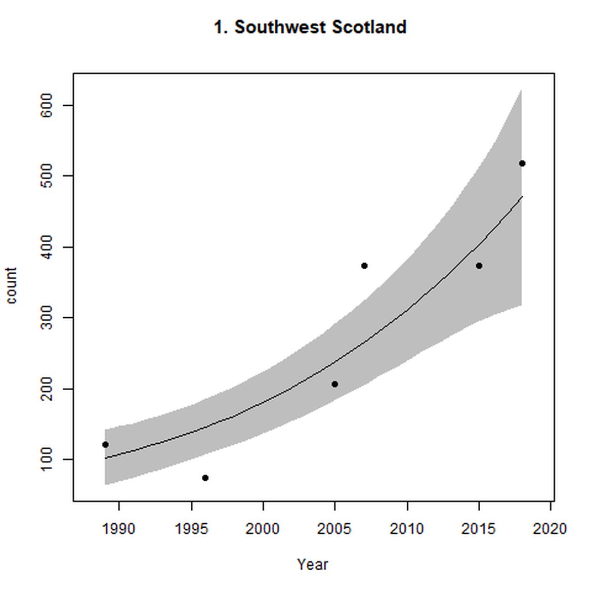
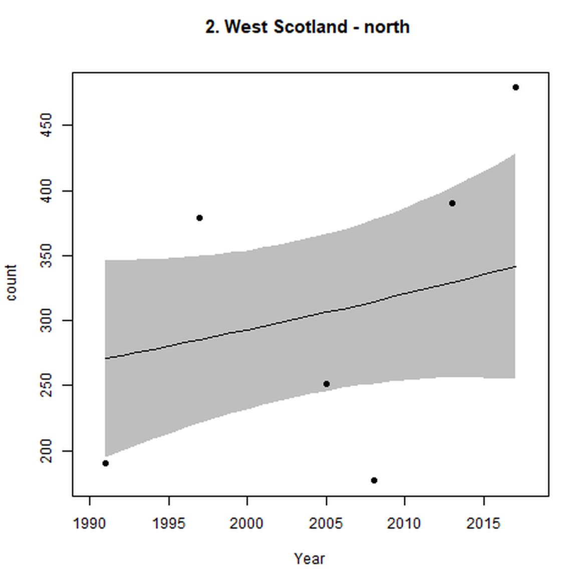
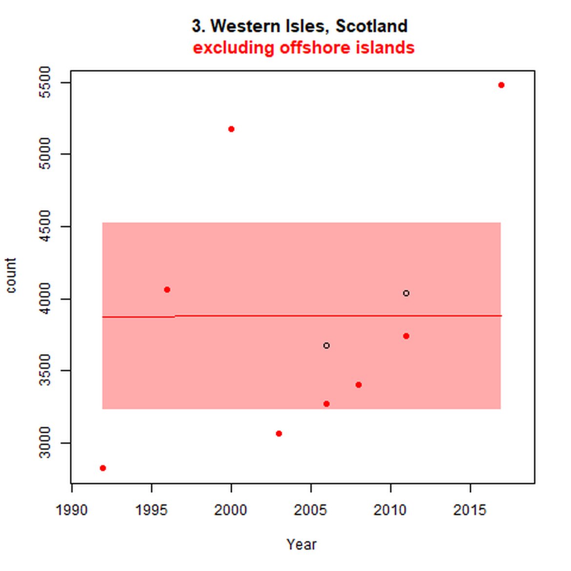
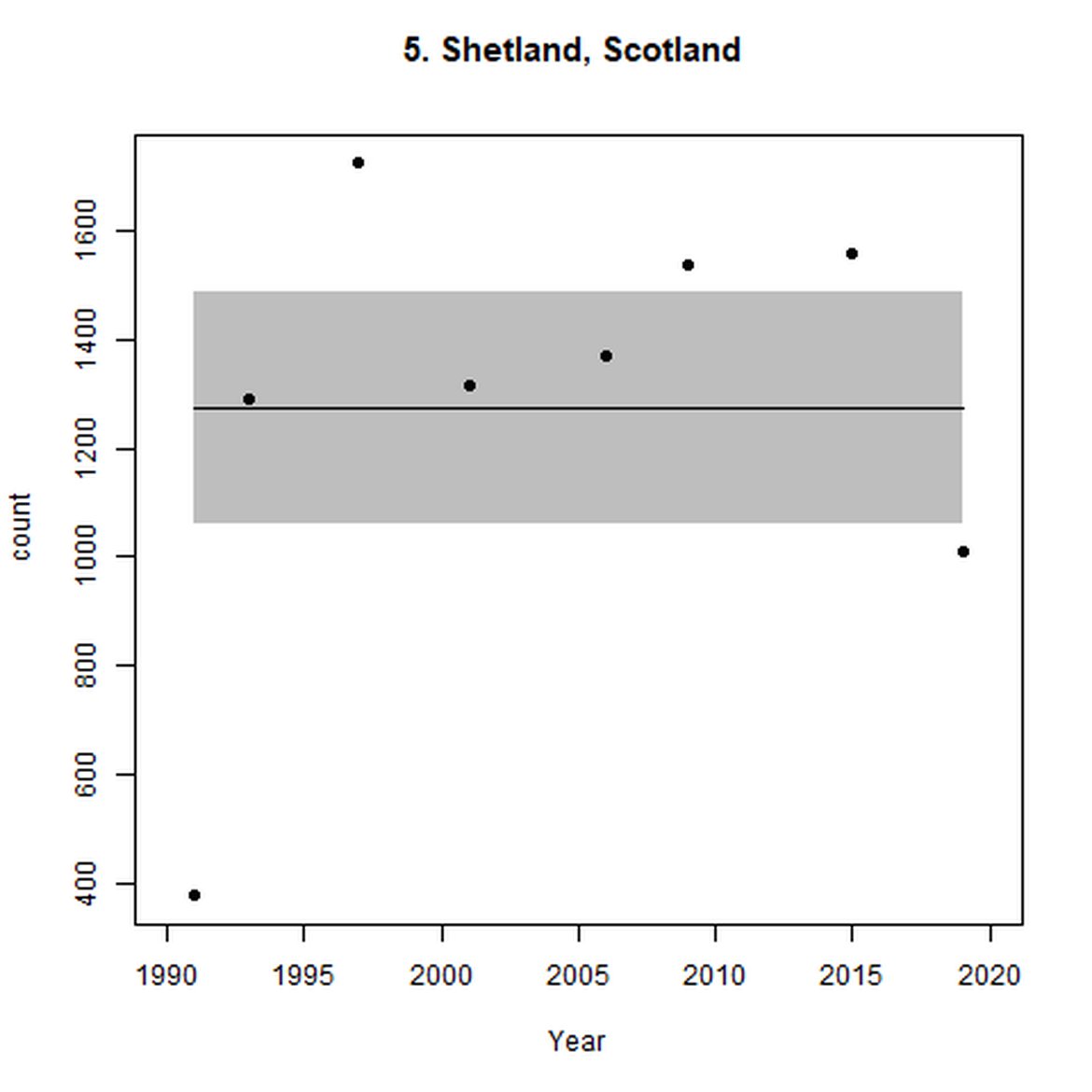
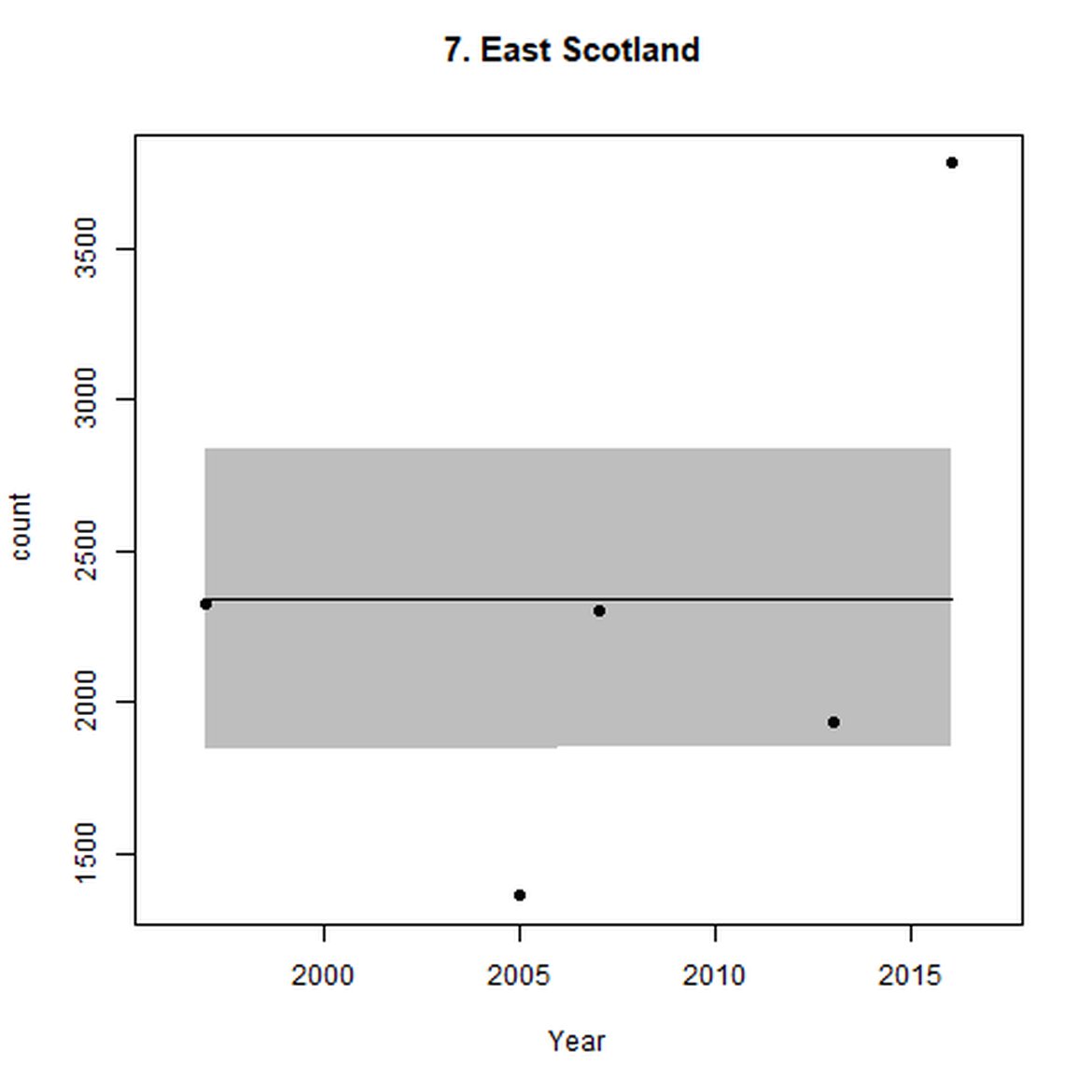
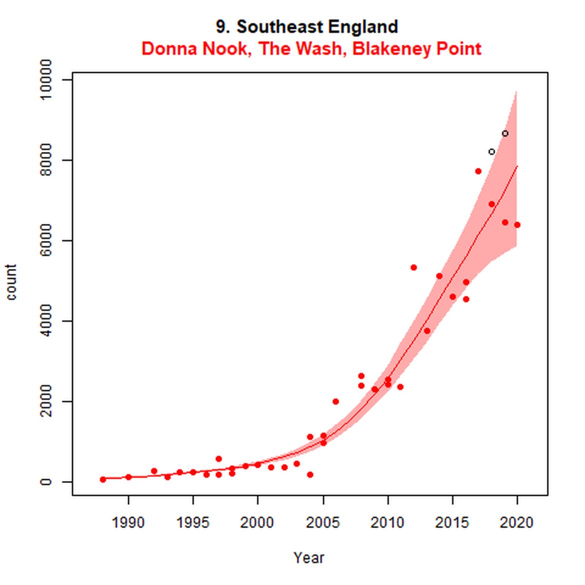
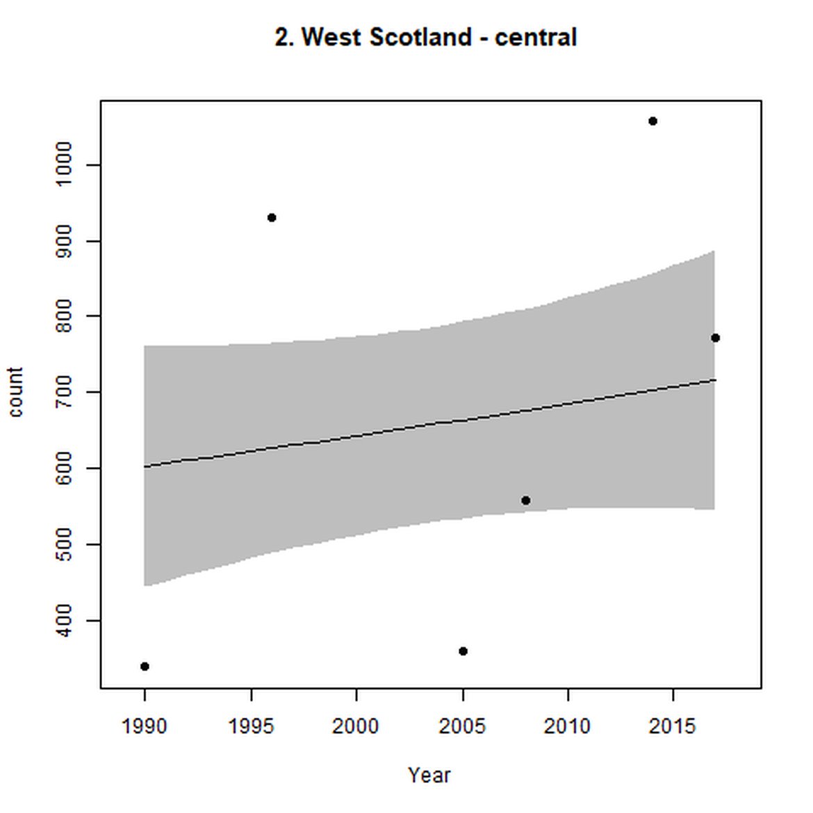
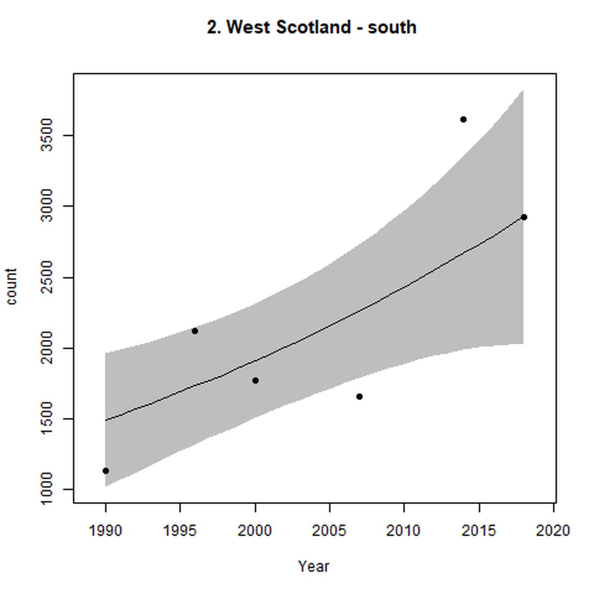
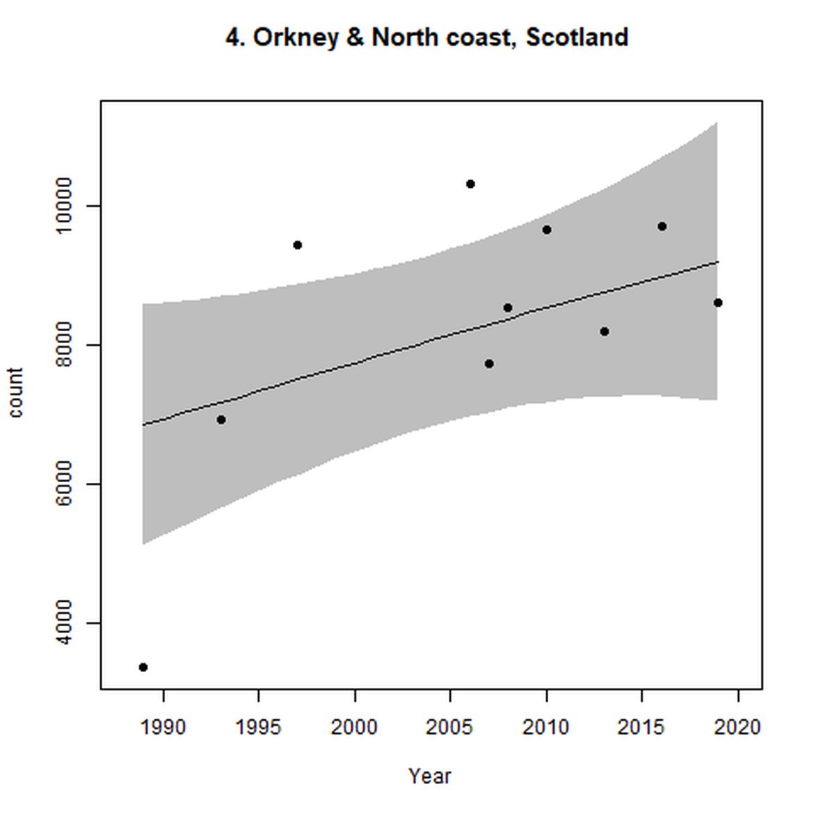
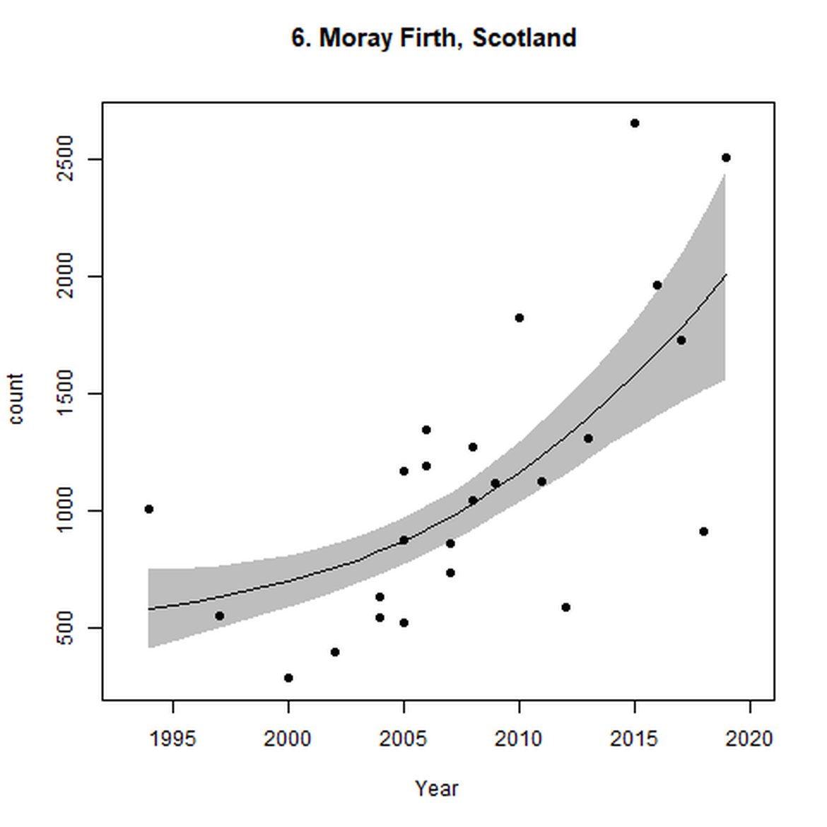
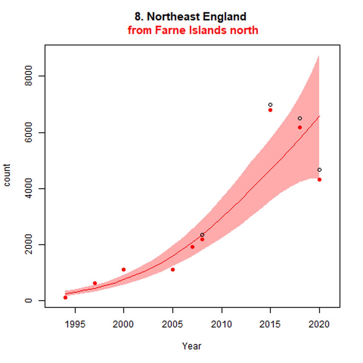
Figure d: Trends in grey seal abundance from surveys of grey seals during the harbour seal moult (summer) in Assessment Units 1 – 15.
Points denote observed numbers of seals. Grey vertical lines denote the years extracted as part of the long- and short-term assessments (baseline year, 2014 and 2019). 80% confidence intervals are illustrated in grey. Filled circles represent the values used to fit the trend. If a subset of the sub-AU was used to fit the trend (red), any full sub-AU counts are shown as open circles. West Scotland sub-AU was split further into three, to maximise the data available.
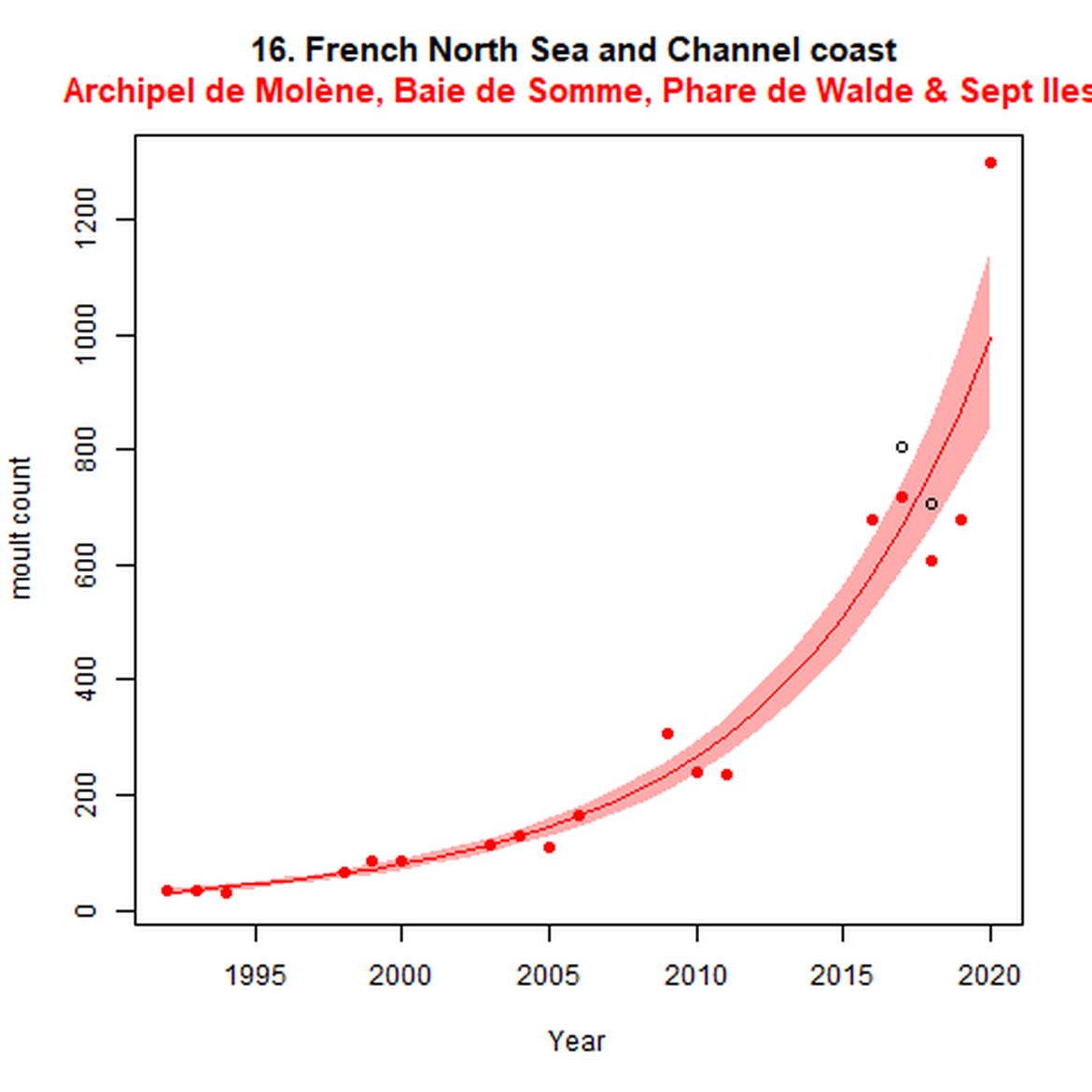
Figure e: Trends in grey seal abundance from surveys of grey seals during the grey seal moult (early spring) in Assessment Units 16 - 18.
Points denote observed numbers of seals. Grey vertical lines denote the years extracted as part of the long- and short-term assessments (baseline year, 2014 and 2019). 80% confidence intervals are illustrated in grey. Filled circles represent the values used to fit the trend. If a subset of the sub-AU was used to fit the trend (red), any full sub-AU counts are shown as open circles.
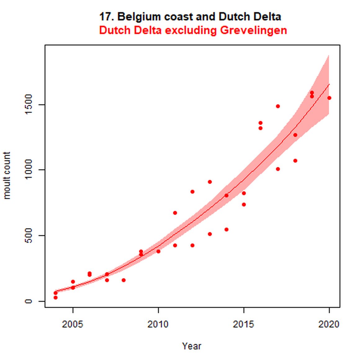
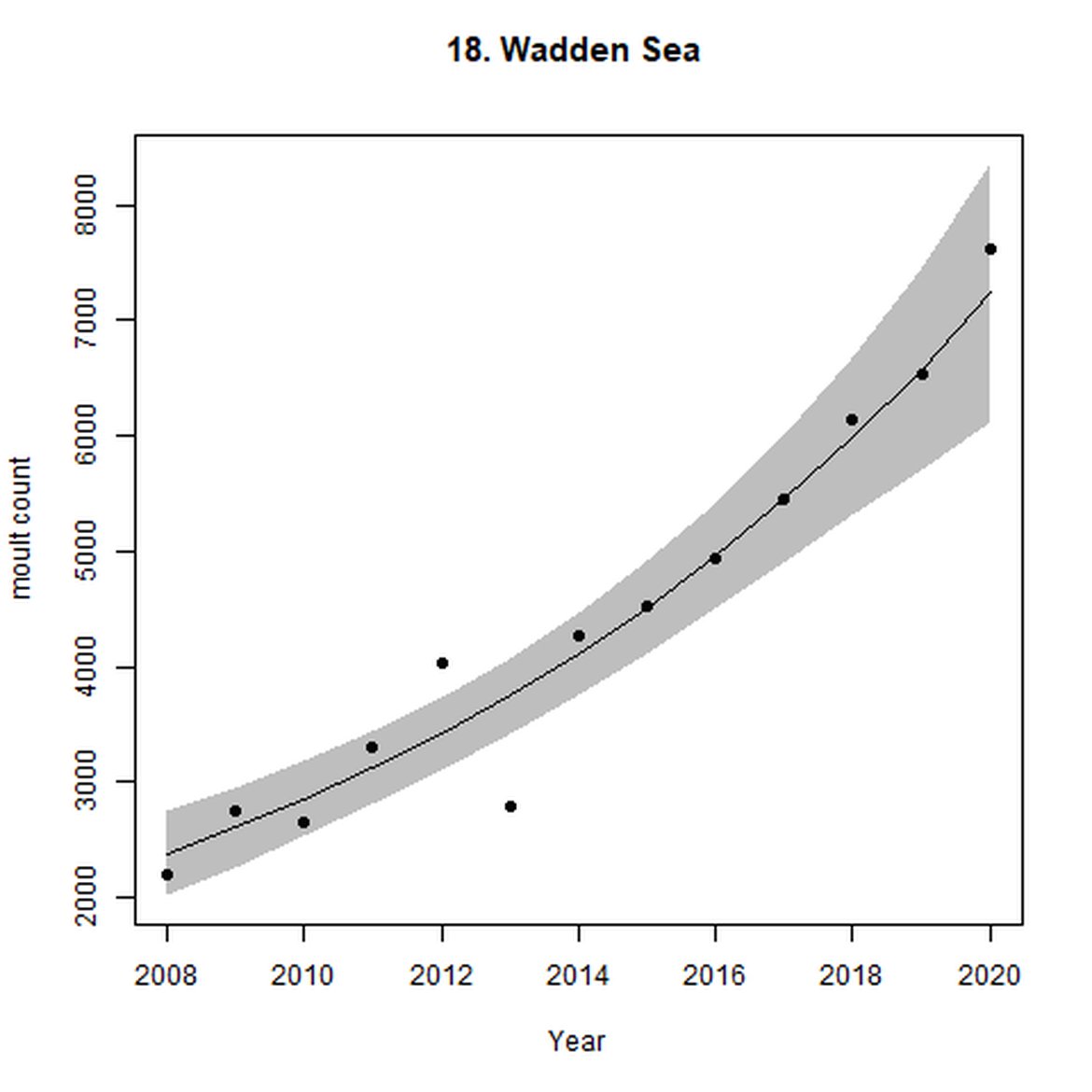
Table a: Sub-AUs and their contribution to the analysis. Note for some years and sub-AUs, multiple counts were available (sub-AUs 6, 9 and 19) and thus Ncounts does not equate to number of years of data. Counts provided for subAUs 16 and 18 were means of multiple counts.
| SubAU | Count type | Contribution | Years of data | Ncounts | Most recent count | Comment | ||
| Number | Name | First | Last | |||||
| 1 | Southwest Scotland | Summer | Modelled | 1989 | 2018 | 6 | 517 | |
| 2 | West Scotland | Summer | Modelled | 1990/1991 | 2017/2018 | 6 | 4174 | |
| 3 | Western Isles | Summer | Modelled | 1992 | 2017 | 8 | 5478 | Subset (93% of count in 2011 – more recent full subAU count) |
| 4 | North Coast & Orkney | Summer | Modelled | 1989 | 2019 | 10 | 8599 | |
| 5 | Shetland | Summer | Modelled | 1991 | 2019 | 8 | 1009 | |
| 6 | Moray Firth | Summer | Modelled | 1994 | 2019 | 21 | 2513 | |
| 7 | East Scotland | Summer | Modelled | 1997 | 2016 | 5 | 3782 | |
| 8 | Northeast England | Summer | Modelled | 1994 | 2020 | 9 | 4703 | |
| 9 | Southeast England | Summer | Modelled | 1988 | 2020 | 30 | 6387 | Subset (74% of count in 2019 – most recent full subAU count) |
| 10 | South England | Summer | Excluded | <501 | ||||
| 11 | Southwest England | Summer | Excluded | c.6251 | No times-series available | |||
| 12 | Wales | Summer | Excluded | c.8001 | No times-series | |||
| 13 | Northwest England | Summer | Excluded | c.3001 | No times-series | |||
| 14 | Northern Ireland | Summer | Modelled | 2002 | 2018 | 7 | 432 | Subset (86% of count in 2019 – most recent full subAU count) |
| 15 | Ireland | Summer | Modelled | 2003 | 2017 | 3 | 3698 | |
| 16 | French North Sea & Channel Coast | Moult | Modelled | 1992 | 2020 | 18 | 1297 | Subset (86% of count in 2018 full subAU count) |
| 17 | Belgium Coast & Dutch Delta | Moult | Modelled | 2004 | 2020 | 32 | 1550 | Subset (Dutch data only and excluding Grevelingen (0-2 seals) |
| 18 | Wadden Sea | Moult | Modelled | 2008 | 2020 | 13 | 7622 | |
1Russell & Morris 2020
Grey Seal Distribution
Distribution of grey seal haul-out sites was analysed using the 25 AUs (Figure a). Shift indexes remain high across the long- and short-term windows indicating that seals have remained in the same locations over time, while the occupancy (their spread across the available habitat) has enlarged in several AUs (Figure f).
Table b: Grey seal summer/moult haul-out distribution change. Numbers given in the occupancy columns are number of cells with percentage of total cells in brackets. Bracketed percentages in long- and short-term occupancy denote the difference in percentage of occupied cells in Years A-C. For cells denoted with * polygons were used instead of cells (AU 17). AU 18b refers to Wadden Sea Netherlands data only.
The Ncells value is essential to consider when interpreting occupancy percentage changes and shift indexes. A percentage change in an AU with a low Ncells value must be regarded as not equivalent to a similar percentage change in an AU with a high Ncells value. That is, an AU with an Ncells value of 4, may produce a 50% increase in occupancy output if an additional two 15 km2 grid cells are occupied in the next focal year. This would not be considered as a significant increase in area use when compared to an AU with an Ncells value of 50, whereby occupancy would need to increase by 25 further 15 km2 grid cells to calculate a similar 50% increase in occupancy.
| Occupied Cells | Long Term (A-C) Occupancy Change | Short Term (B-C) Occupancy Change | ||||||||||||
| AU | Name | Ncells | Year A | Year B | Year C | Year A (%) | Year B (%) | Year C (%) | Change (%) | Shift Index | Change (%) | Shift Index | Data | Comments |
| 1 | Southwest Scotland | 64 | 1996 | 2015 | 2018 | 3 (4,69 %) | 28 (43,75%) | 29 (45,31%) | 26 (40,63%) | 0,13 | 1 (1,56%) | 0,77 | summer | |
| 2 | West Scotland | 119 | 1996-1997 | 2013-2015 | 2017-2018 | 50 (42,02 %) | 85 (71,43%) | 88 (73,95%) | 35 (31,93%) | 0,67 | 3 (2,52%) | 0,9 | summer | |
| 3 | Western Isles | 43 | 1996 | 2011 | 2017 | 35 (81,4%) | 34 (79,07%) | 35 (81,4%) | 0 (0%) | 0,86 | 1 (2,33%) | 0,9 | summer | |
| 4 | North Coast & Orkney | 33 | 1997 | 20013 | 2016 & 2019 | 26 (78,79%) | 26 (78,79%) | 27 (81,81%) | 1 (3,03%) | 0,94 | 1 (3,03%) | 0,98 | summer | |
| 5 | Shetland | 28 | 1997 | 2015 | 2019 | 24 (85,71%) | 23 (82,14%) | 22 (78,57%) | -2 (-7,14%) | 0,83 | -1 (-3,57%) | 0,84 | summer | |
| 6 | Moray Firth | 19 | 1997 | 2013 | 2019 | 4 (21,05%) | 8 (42,11%) | 7 (36,84%) | 3 (15,79%) | 0,73 | -1 (-5,26%) | 0,93 | summer | |
| 7 | East Scotland | 27 | 1997 | 2013 | 2016 & 2019 | 16 (59,26%) | 16 (59,26%) | 17 (62,96%) | 1 (3,7%) | 0,72 | 1 (3,7%) | 0,79 | summer | |
| 8 | Northeast England | 4 | 1997 | 2013 & 2015 | 2018 | 2 (50%) | 3 (75%) | 4 (100%) | 2 (50%) | 0,67 | 1 (25%) | 0,86 | summer | |
| 9 | Southeast England | 54 | 2003 | 2014 | 2019 | 9 (16,67%) | 17 (31,48%) | 21 (38,89%) | 12 (22,22%) | 0,47 | 4 (7,41%) | 0,74 | summer | |
| 10 | South England | NA | NA | NA | NA | NA | NA | NA | NA | NA | NA | NA | NA | |
| 11 | Southwest England | NA | NA | NA | NA | NA | NA | NA | NA | NA | NA | NA | NA | |
| 12 | Wales | NA | NA | NA | NA | NA | NA | NA | NA | NA | NA | NA | NA | |
| 13 | Northwest England | NA | 1996 | 2015 | 2018 | NA | NA | NA | NA | 1 | NA | 1 | summer | no seals |
| 14 | Northern Ireland | 30 | 2002 | 2011 | 2018 | 7 (23,33%) | 15 (50%) | 20 (66,67%) | 13 (43,33%) | 0,52 | 5 (16,67%) | 0,86 | summer | |
| 15 | Republic of Ireland | 200 | 2003 | 2011-2012 | 2017-2018 | 68 (34%) | 94 (47%) | 101 (50,5%) | 41 (16,5%) | 0,69 | 7 (3,5%) | 0,8 | summer | |
| 16 | French North Sea & Channel Coast | 5 | 2002-2003 | 2011-2012 | 2019 | 4 (80%) | 4 (80%) | 5 (100%) | 1 (20%) | 0,89 | 1 (20%) | 0,89 | moult | |
| 17 | Belgium Coast & Dutch Delta | 3* | 2004 | 2014 | 2019 | 1 (33,33%) | 1 (33,33%) | 2 (66,67%) | 1 (33,33%) | 0,67 | 1 (33,33%) | 0,67 | moult | 15 km2 grid not used for AU 17 - 3 large polygons provided by Netherlands used instead. |
| 18 | Wadden Sea | 43 | 2008 | 2014 | 2019 | 33 (76,74%) | 31 (72,09%) | 35 (81,4%) | 2 (4,65%) | 0,94 | 4 (9,3%) | 0,94 | moult | Danish data excluded as summer pre 2015 and moult 2015-2020. German and NL data included. Trend driven by German data |
| 18b | Wadden Sea-NL | 14 | 2002 | 2014 | 2019 | 14 (100%) | 14 (100%) | 14 (100%) | 0 (0%) | 1 | 0 (0%) | 1 | moult | NL data only as interim |
| 19 | Limfjorden | 7 | 1999 | 2014 | 2019 | 0 (0%) | 1 (14,29%) | 2 (28,57%) | 2 (28,57%) | 0 | 1 (14,29%) | 0,67 | summer | |
| 20 | Kattegat | 9 | 1992 | 2014 | 2019 | 3 (33,33%) | 4 (44,44%) | 5 (55,56%) | 2 (22,22%) | 0,5 | 1 (11,11%) | 0,89 | summer | Swedish Kattegat not covered |
| 21 | Iceland | NA | NA | NA | NA | NA | NA | NA | NA | NA | NA | NA | NA | |
| 22 | Skagerrak | NA | NA | NA | NA | NA | NA | NA | NA | NA | NA | NA | NA | |
| 23 | Norway MA1 | NA | NA | NA | NA | NA | NA | NA | NA | NA | NA | NA | NA | |
| 24 | Norway MA2 | NA | NA | NA | NA | NA | NA | NA | NA | NA | NA | NA | NA | |
| 25 | Norway MA3 | NA | NA | NA | NA | NA | NA | NA | NA | NA | NA | NA | NA | |
 and (b) show count data (red = absence, blue = presence), AU is shown in light blue. (c) shows presence / absence data aggregated to 15km² cells (occupancy = 40.63, shift = 0.13, n. cells = 64).")
AU1 Long Term analysis. Maps (a) and (b) show count data (red = absence, blue = presence), AU is shown in light blue. (c) shows presence / absence data aggregated to 15km² cells (occupancy = 40.63, shift = 0.13, n. cells = 64).
 and (b) show count data (red = absence, blue = presence), AU is shown in light blue. (c) shows presence / absence data aggregated to 15km² cells (occupancy = 1.56, shift = 0.77, n. cells = 64).")
AU1 Short Term analysis. Maps (a) and (b) show count data (red = absence, blue = presence), AU is shown in light blue. (c) shows presence / absence data aggregated to 15km² cells (occupancy = 1.56, shift = 0.77, n. cells = 64).
 and (b) show count data (red = absence, blue = presence), AU is shown in light blue. (c) shows presence / absence data aggregated to 15km² cells (occupancy = 31.93, shift = 0.67, n. cells = 119).")
AU2 Long Term analysis. Maps (a) and (b) show count data (red = absence, blue = presence), AU is shown in light blue. (c) shows presence / absence data aggregated to 15km² cells (occupancy = 31.93, shift = 0.67, n. cells = 119).
 and (b) show count data (red = absence, blue = presence), AU is shown in light blue. (c) shows presence / absence data aggregated to 15km² cells (occupancy = 2.52, shift = 0.9, n. cells = 119).")
AU2 Short Term analysis. Maps (a) and (b) show count data (red = absence, blue = presence), AU is shown in light blue. (c) shows presence / absence data aggregated to 15km² cells (occupancy = 2.52, shift = 0.9, n. cells = 119).
 and (b) show count data (red = absence, blue = presence), AU is shown in light blue. (c) shows presence / absence data aggregated to 15km² cells (occupancy = 0, shift = 0.89, n. cells = 43).")
AU3 Long Term analysis. Maps (a) and (b) show count data (red = absence, blue = presence), AU is shown in light blue. (c) shows presence / absence data aggregated to 15km² cells (occupancy = 0, shift = 0.89, n. cells = 43).
 and (b) show count data (red = absence, blue = presence), AU is shown in light blue. (c) shows presence / absence data aggregated to 15km² cells (occupancy = 2.33, shift = 0.9, n. cells = 43).")
AU3 Short Term analysis. Maps (a) and (b) show count data (red = absence, blue = presence), AU is shown in light blue. (c) shows presence / absence data aggregated to 15km² cells (occupancy = 2.33, shift = 0.9, n. cells = 43).
 and (b) show count data (red = absence, blue = presence), AU is shown in light blue. (c) shows presence / absence data aggregated to 15km² cells (occupancy = 3.03, shift = 0.94, n. cells = 33).")
AU4 Long Term analysis. Maps (a) and (b) show count data (red = absence, blue = presence), AU is shown in light blue. (c) shows presence / absence data aggregated to 15km² cells (occupancy = 3.03, shift = 0.94, n. cells = 33).
 and (b) show count data (red = absence, blue = presence), AU is shown in light blue. (c) shows presence / absence data aggregated to 15km² cells (occupancy = 3.03, shift = 0.98, n. cells = 33).")
AU4 Short Term analysis. Maps (a) and (b) show count data (red = absence, blue = presence), AU is shown in light blue. (c) shows presence / absence data aggregated to 15km² cells (occupancy = 3.03, shift = 0.98, n. cells = 33).
 and (b) show count data (red = absence, blue = presence), AU is shown in light blue. (c) shows presence / absence data aggregated to 15km² cells (occupancy = -7.14, shift = 0.83, n. cells = 28).")
AU5 Long Term analysis. Maps (a) and (b) show count data (red = absence, blue = presence), AU is shown in light blue. (c) shows presence / absence data aggregated to 15km² cells (occupancy = -7.14, shift = 0.83, n. cells = 28).
 and (b) show count data (red = absence, blue = presence), AU is shown in light blue. (c) shows presence / absence data aggregated to 15km² cells (occupancy = -3.57, shift = 0.84, n. cells = 28).")
AU5 Short Term analysis. Maps (a) and (b) show count data (red = absence, blue = presence), AU is shown in light blue. (c) shows presence / absence data aggregated to 15km² cells (occupancy = -3.57, shift = 0.84, n. cells = 28).
 and (b) show count data (red = absence, blue = presence), AU is shown in light blue. (c) shows presence / absence data aggregated to 15km² cells (occupancy = 15.79, shift = 0.73, n. cells = 19).")
AU6 Long Term analysis. Maps (a) and (b) show count data (red = absence, blue = presence), AU is shown in light blue. (c) shows presence / absence data aggregated to 15km² cells (occupancy = 15.79, shift = 0.73, n. cells = 19).
 and (b) show count data (red = absence, blue = presence), AU is shown in light blue. (c) shows presence / absence data aggregated to 15km² cells (occupancy = -5.26, shift = 0.93, n. cells = 19).")
AU6 Short Term analysis. Maps (a) and (b) show count data (red = absence, blue = presence), AU is shown in light blue. (c) shows presence / absence data aggregated to 15km² cells (occupancy = -5.26, shift = 0.93, n. cells = 19).
 and (b) show count data (red = absence, blue = presence), AU is shown in light blue. (c) shows presence / absence data aggregated to 15km² cells (occupancy = 3.7, shift = 0.73, n. cells = 27).")
AU7 Long Term analysis. Maps (a) and (b) show count data (red = absence, blue = presence), AU is shown in light blue. (c) shows presence / absence data aggregated to 15km² cells (occupancy = 3.7, shift = 0.73, n. cells = 27).
 and (b) show count data (red = absence, blue = presence), AU is shown in light blue. (c) shows presence / absence data aggregated to 15km² cells (occupancy = 3.7, shift = 0.79, n. cells = 27).")
AU7 Short Term analysis. Maps (a) and (b) show count data (red = absence, blue = presence), AU is shown in light blue. (c) shows presence / absence data aggregated to 15km² cells (occupancy = 3.7, shift = 0.79, n. cells = 27).
 and (b) show count data (red = absence, blue = presence), AU is shown in light blue. (c) shows presence / absence data aggregated to 15km² cells (occupancy = 50, shift = 0.67, n. cells = 4).")
AU8 Long Term analysis. Maps (a) and (b) show count data (red = absence, blue = presence), AU is shown in light blue. (c) shows presence / absence data aggregated to 15km² cells (occupancy = 50, shift = 0.67, n. cells = 4).
 and (b) show count data (red = absence, blue = presence), AU is shown in light blue. (c) shows presence / absence data aggregated to 15km² cells (occupancy = 25, shift = 0.86, n. cells = 4).")
AU8 Short Term analysis. Maps (a) and (b) show count data (red = absence, blue = presence), AU is shown in light blue. (c) shows presence / absence data aggregated to 15km² cells (occupancy = 25, shift = 0.86, n. cells = 4).
 and (b) show count data (red = absence, blue = presence), AU is shown in light blue. (c) shows presence / absence data aggregated to 15km² cells (occupancy = 22.22, shift = 0.47, n. cells = 54).")
AU9 Long Term analysis. Maps (a) and (b) show count data (red = absence, blue = presence), AU is shown in light blue. (c) shows presence / absence data aggregated to 15km² cells (occupancy = 22.22, shift = 0.47, n. cells = 54).
 and (b) show count data (red = absence, blue = presence), AU is shown in light blue. (c) shows presence / absence data aggregated to 15km² cells (occupancy = 7.41, shift = 0.74, n. cells = 54).")
AU9 Short Term analysis. Maps (a) and (b) show count data (red = absence, blue = presence), AU is shown in light blue. (c) shows presence / absence data aggregated to 15km² cells (occupancy = 7.41, shift = 0.74, n. cells = 54).
 and (b) show count data (red = absence, blue = presence), AU is shown in light blue. (c) shows presence / absence data aggregated to 15km² cells (occupancy = 43.33, shift = 0.52, n. cells = 30).")
AU14 Short Term analysis. Maps (a) and (b) show count data (red = absence, blue = presence), AU is shown in light blue. (c) shows presence / absence data aggregated to 15km² cells (occupancy = 43.33, shift = 0.52, n. cells = 30).
 and (b) show count data (red = absence, blue = presence), AU is shown in light blue. (c) shows presence / absence data aggregated to 15km² cells (occupancy = 16.67, shift = 0.86, n. cells = 30).")
AU14 Short Term analysis. Maps (a) and (b) show count data (red = absence, blue = presence), AU is shown in light blue. (c) shows presence / absence data aggregated to 15km² cells (occupancy = 16.67, shift = 0.86, n. cells = 30).
 and (b) show count data (red = absence, blue = presence), AU is shown in light blue. (c) shows presence / absence data aggregated to 15km² cells (occupancy = 16.5, shift = 0.69, n. cells = 200).")
AU15 Long Term analysis. Maps (a) and (b) show count data (red = absence, blue = presence), AU is shown in light blue. (c) shows presence / absence data aggregated to 15km² cells (occupancy = 16.5, shift = 0.69, n. cells = 200).
 and (b) show count data (red = absence, blue = presence), AU is shown in light blue. (c) shows presence / absence data aggregated to 15km² cells (occupancy = 3.5, shift = 0.8, n. cells = 200).")
AU15 Short Term analysis. Maps (a) and (b) show count data (red = absence, blue = presence), AU is shown in light blue. (c) shows presence / absence data aggregated to 15km² cells (occupancy = 3.5, shift = 0.8, n. cells = 200).
 and (b) show count data (red = absence, blue = presence), AU is shown in light blue. (c) shows presence / absence data aggregated to 15km² cells (occupancy = 20, shift = 0.89, n. cells = 5).")
AU16 Long Term analysis. Maps (a) and (b) show count data (red = absence, blue = presence), AU is shown in light blue. (c) shows presence / absence data aggregated to 15km² cells (occupancy = 20, shift = 0.89, n. cells = 5).
 and (b) show count data (red = absence, blue = presence), AU is shown in light blue. (c) shows presence / absence data aggregated to 15km² cells (occupancy = 20, shift = 0.89, n. cells = 5).")
AU16 Short Term analysis. Maps (a) and (b) show count data (red = absence, blue = presence), AU is shown in light blue. (c) shows presence / absence data aggregated to 15km² cells (occupancy = 20, shift = 0.89, n. cells = 5).
 and (b) show count data (red = absence, blue = presence), AU is shown in light blue. (c) shows presence / absence data per survey polygon (occupancy = 33.33, shift = 0.67, n. polygons = 3). It was not possible to aggregate these data to 15 km² cells given the large size of the survey polygons.")
AU17 Long Term analysis. Maps (a) and (b) show count data (red = absence, blue = presence), AU is shown in light blue. (c) shows presence / absence data per survey polygon (occupancy = 33.33, shift = 0.67, n. polygons = 3). It was not possible to aggregate these data to 15 km² cells given the large size of the survey polygons.
 and (b) show count data (red = absence, blue = presence), AU is shown in light blue. (c) shows presence / absence data per survey polygon (occupancy = 33.33, shift = 0.67, n. polygons = 3). It was not possible to aggregate these data to 15 km² cells given the large size of the survey polygons.")
AU17 Short Term analysis. Maps (a) and (b) show count data (red = absence, blue = presence), AU is shown in light blue. (c) shows presence / absence data per survey polygon (occupancy = 33.33, shift = 0.67, n. polygons = 3). It was not possible to aggregate these data to 15 km² cells given the large size of the survey polygons.
 and (b) show count data (red = absence, blue = presence), AU is shown in light blue. German survey effort cells are shown in red (only areas that overlapped with the coast were considered to have been surveyed). (c) shows presence / absence data aggregated to 15km² cells (occupancy = 4.65, shift = 0.94, n. cells = 43).")
AU18 Long Term analysis. Maps (a) and (b) show count data (red = absence, blue = presence), AU is shown in light blue. German survey effort cells are shown in red (only areas that overlapped with the coast were considered to have been surveyed). (c) shows presence / absence data aggregated to 15km² cells (occupancy = 4.65, shift = 0.94, n. cells = 43).
 and (b) show count data (red = absence, blue = presence), AU is shown in light blue. German survey effort polygons are shown in red (only areas that overlapped with the coast were considered to have been surveyed). (c) shows presence / absence data aggregated to 15km² cells (occupancy = 9.3, shift = 0.94, n. cells = 43).")
AU18 Short Term analysis. Maps (a) and (b) show count data (red = absence, blue = presence), AU is shown in light blue. German survey effort polygons are shown in red (only areas that overlapped with the coast were considered to have been surveyed). (c) shows presence / absence data aggregated to 15km² cells (occupancy = 9.3, shift = 0.94, n. cells = 43).
 and (b) show count data (red = absence, blue = presence), AU is shown in light blue. (c) shows presence / absence data aggregated to 15km² cells (occupancy = 28.57, shift = 0, n. cells = 7).")
AU19 Long Term analysis. Maps (a) and (b) show count data (red = absence, blue = presence), AU is shown in light blue. (c) shows presence / absence data aggregated to 15km² cells (occupancy = 28.57, shift = 0, n. cells = 7).
 and (b) show count data (red = absence, blue = presence), AU is shown in light blue. (c) shows presence / absence data aggregated to 15km² cells (occupancy = 14.29, shift = 0.67, n. cells = 7).")
AU19 Short Term analysis. Maps (a) and (b) show count data (red = absence, blue = presence), AU is shown in light blue. (c) shows presence / absence data aggregated to 15km² cells (occupancy = 14.29, shift = 0.67, n. cells = 7).
 and (b) show count data (red = absence, blue = presence), AU is shown in light blue. (c) shows presence / absence data aggregated to 15km² cells (occupancy = 22.22, shift = 0.5, n. cells = 9).")
AU20 Long Term analysis. Maps (a) and (b) show count data (red = absence, blue = presence), AU is shown in light blue. (c) shows presence / absence data aggregated to 15km² cells (occupancy = 22.22, shift = 0.5, n. cells = 9).
 and (b) show count data (red = absence, blue = presence), AU is shown in light blue. (c) shows presence / absence data aggregated to 15km² cells (occupancy = 11.11, shift = 0.89, n. cells = 9).")
AU20 Short Term analysis. Maps (a) and (b) show count data (red = absence, blue = presence), AU is shown in light blue. (c) shows presence / absence data aggregated to 15km² cells (occupancy = 11.11, shift = 0.89, n. cells = 9).
Figure f: Long- and short-term grey seal distribution change plots using either summer, or spring moult data.
Harbour Seal Abundance
Increases reported as part of this assessment have been punctuated by outbreaks of PDV both since the baseline year of 1992 (i.e., 2002 in the UK), as well as prior to this year (in 1988) which led to population reductions of up to 50% across the AUs. It must be considered therefore, that the 1992 baseline value may be considerably lower than the level indicative of a healthy initial population to compare progress against. This must be considered when scrutinising these trends in abundance.
Trends in abundance were plotted for each AU (Figure g), after which percentage change (mean and 80% confidence intervals) were estimated for each AU over the short- and long-term assessment periods. Of the 25 AUs, 17 units had sufficient data to carry out an assessment of the long-term trends in harbour seal abundance. Of these, two (AU 9 and AU 14) produced inconclusive outputs as a result of the 80% confidence intervals encompassing the threshold value. Seventeen AUs had sufficient data to carry out an assessment of the short-term trends in abundance. Of these, six AUs produced inconclusive outputs (Table c). Assessments were able to be generated at the AU level for three units, but outputs with increased confidence were produced using subset level data. Four AUs were assessed using subsets of data only.
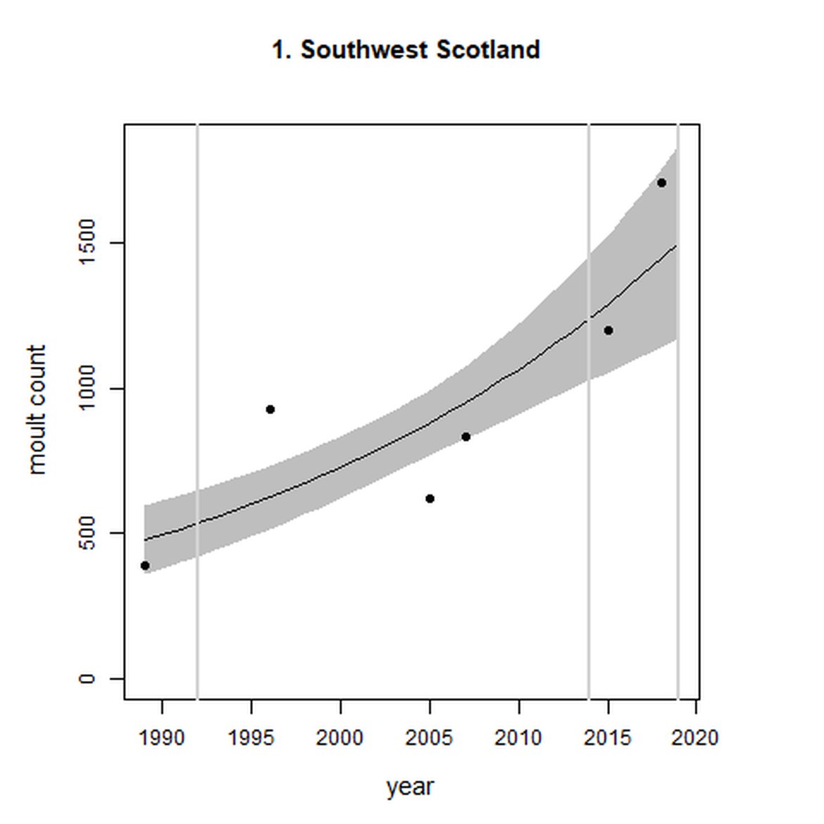
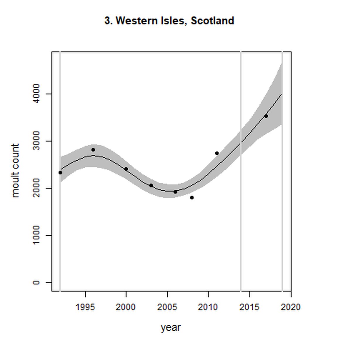
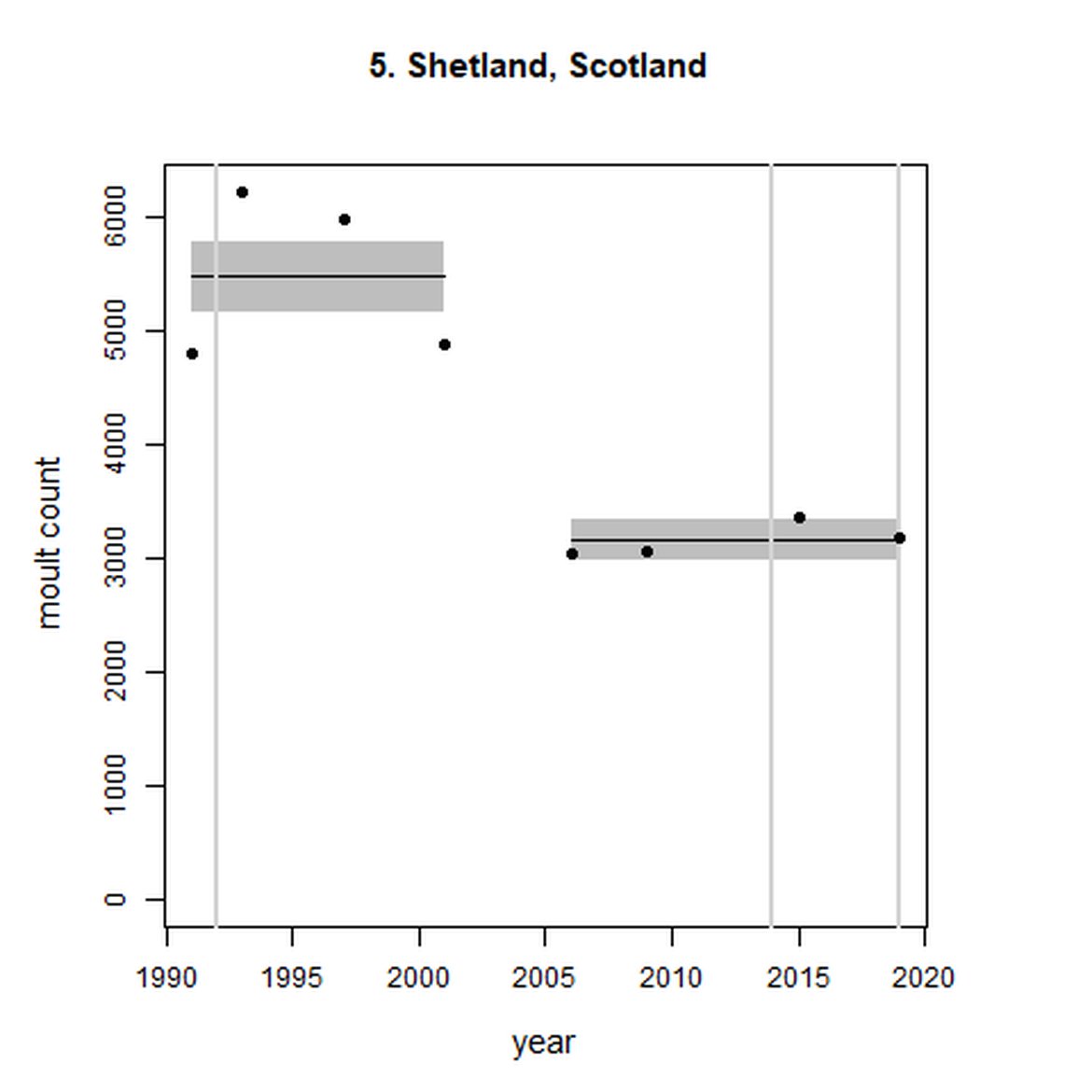
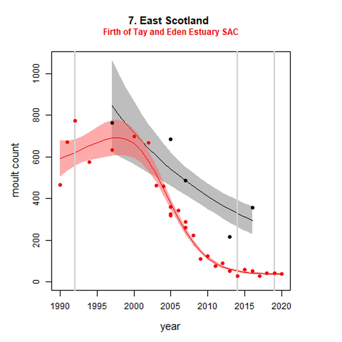
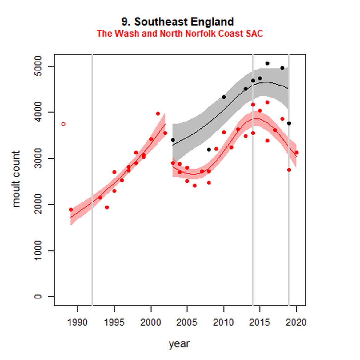
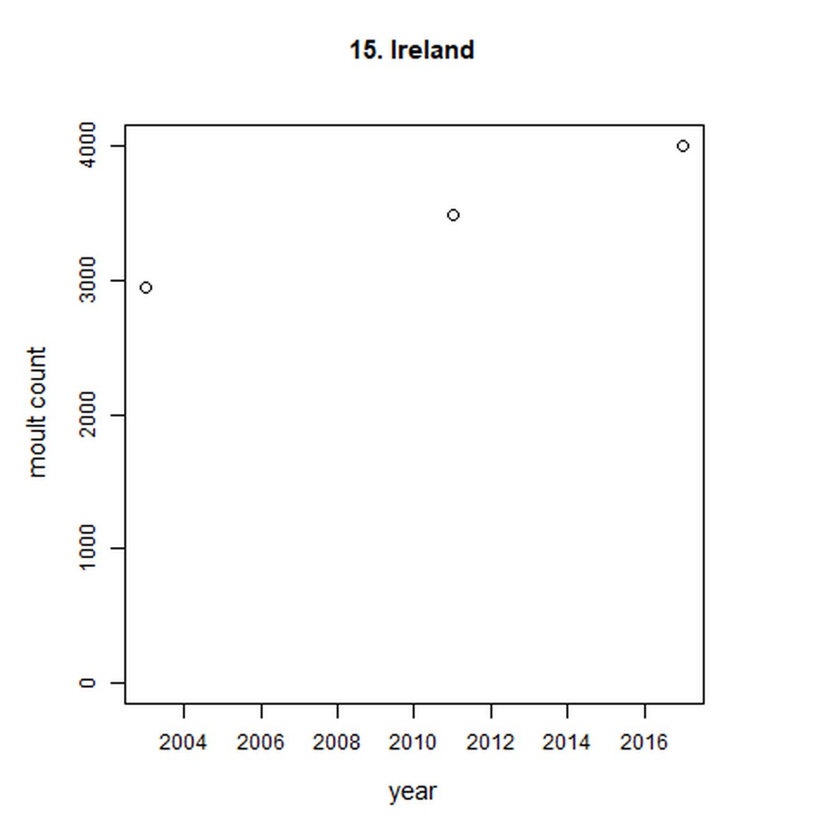
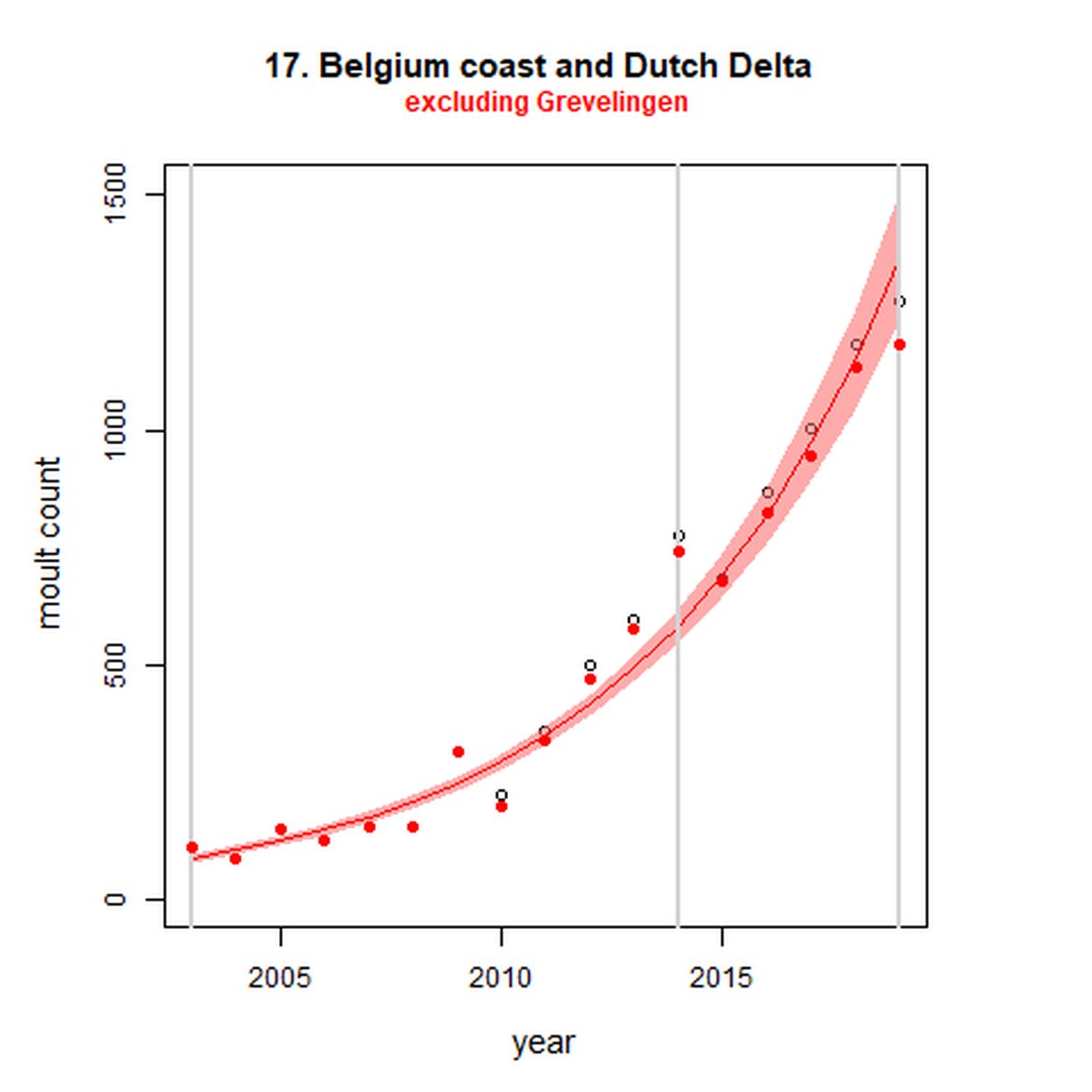
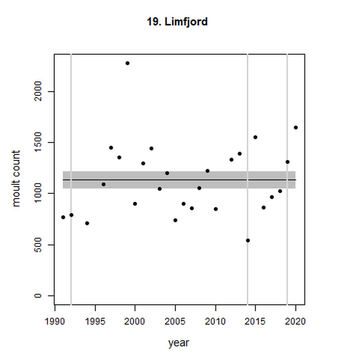
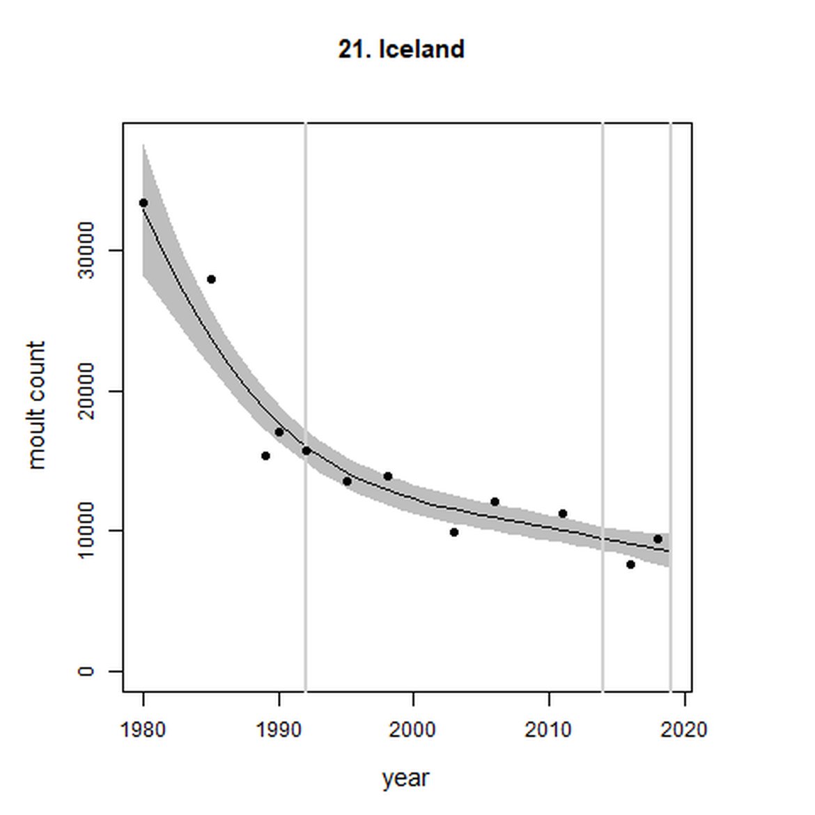
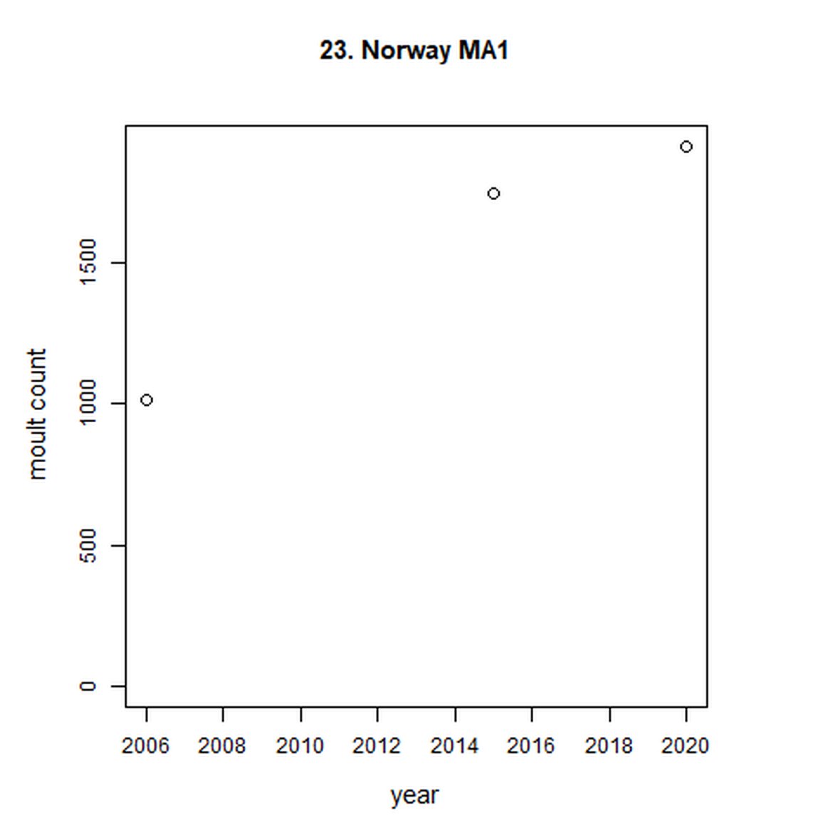
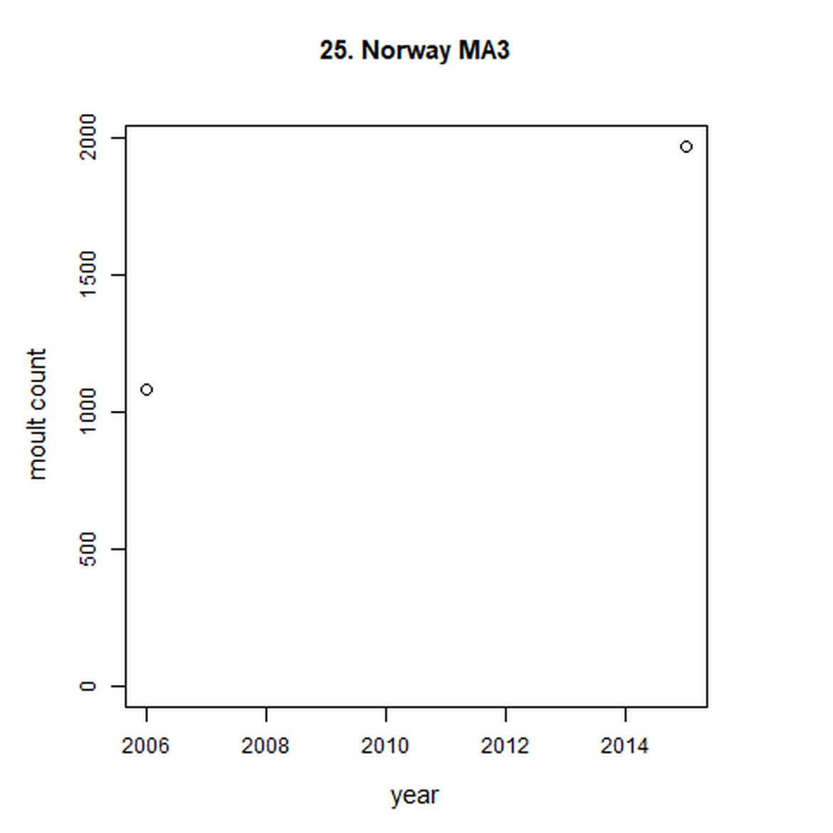
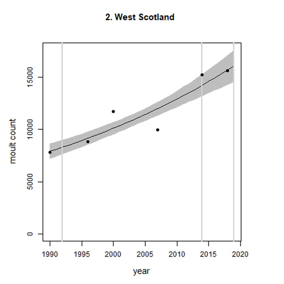
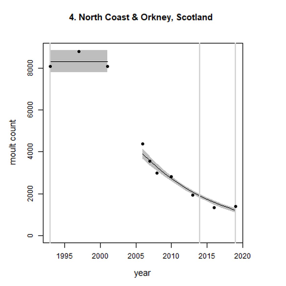
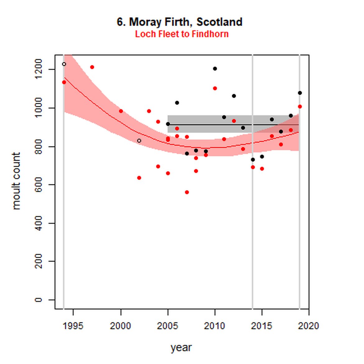
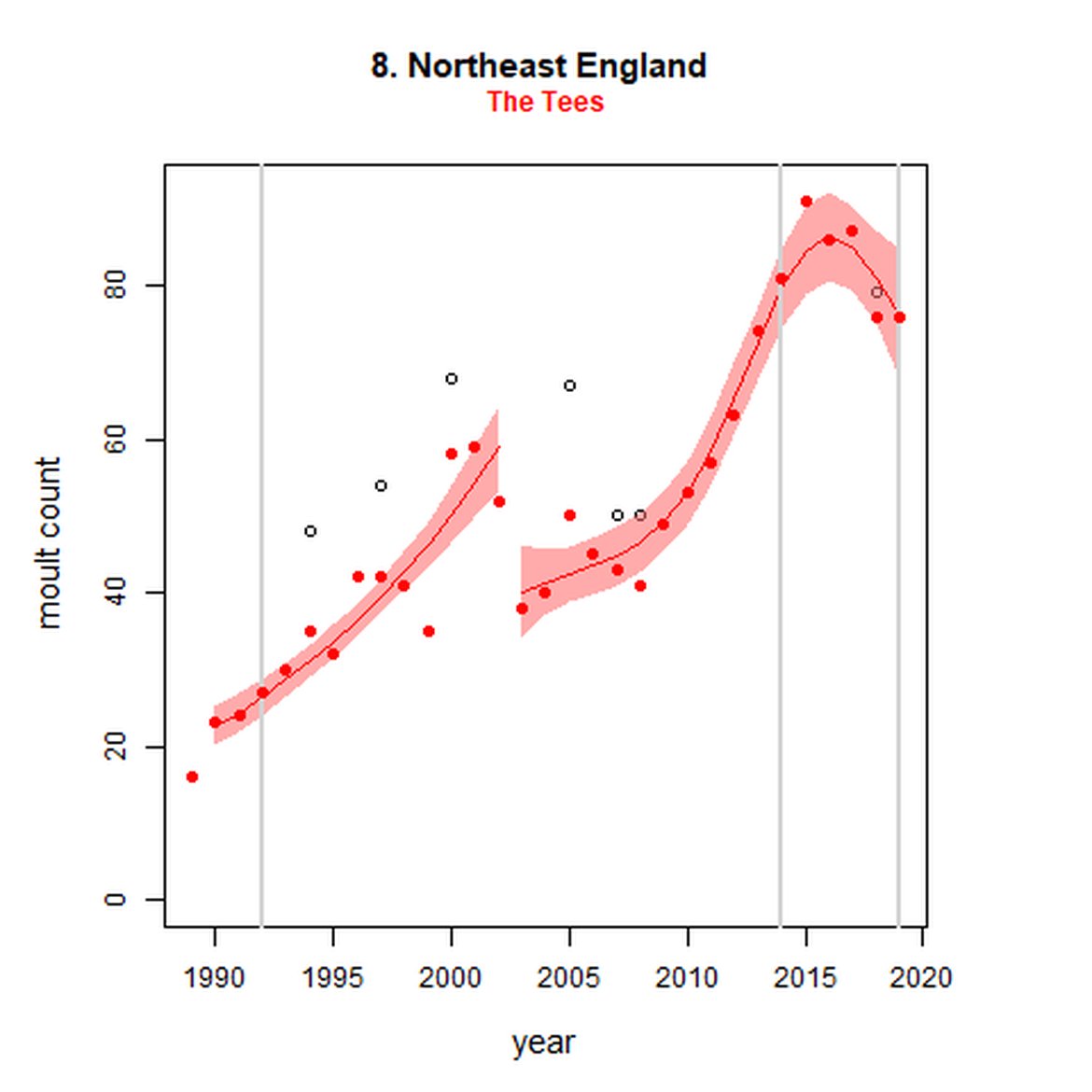
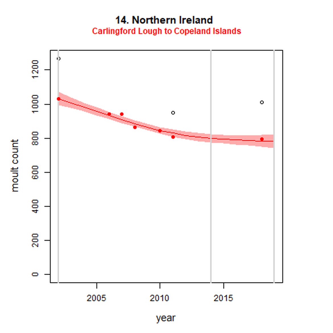
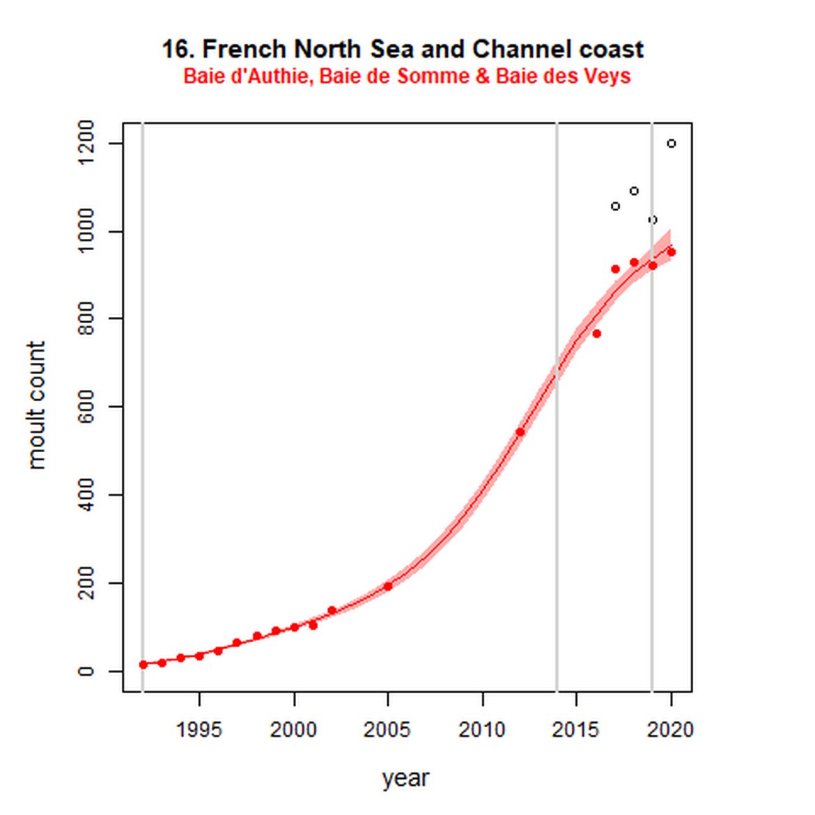
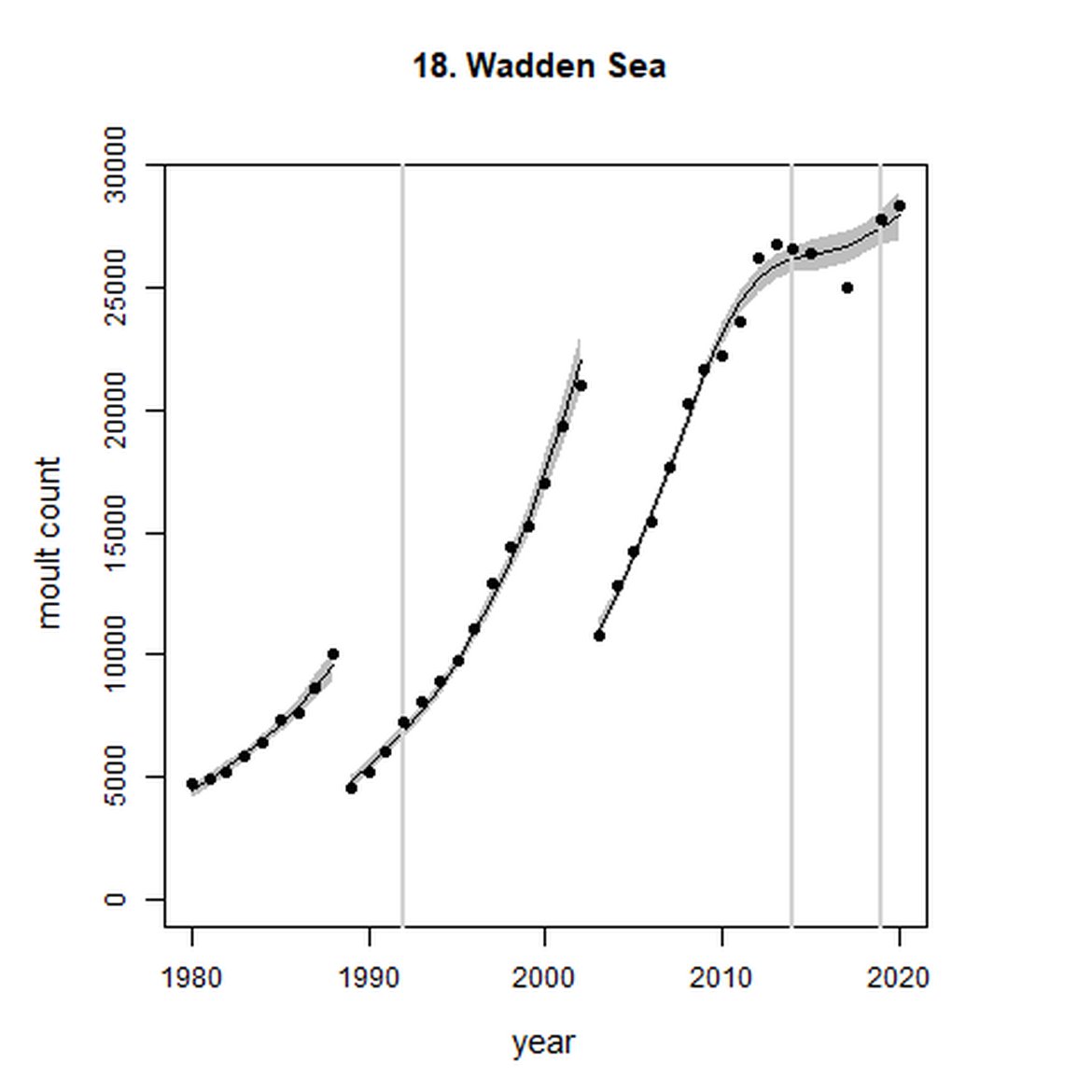
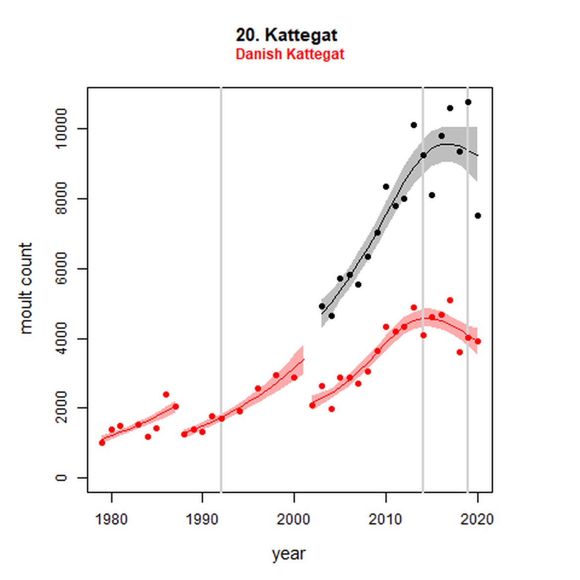
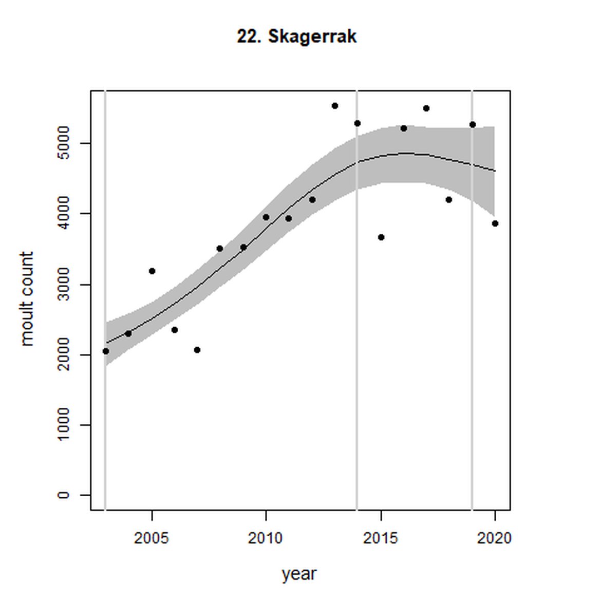
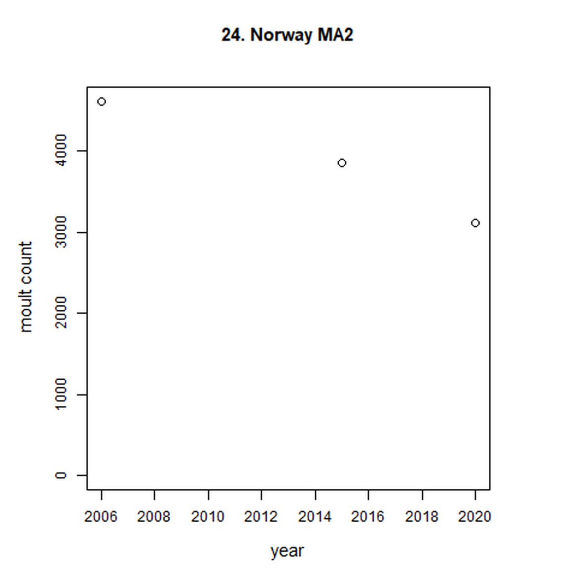
Figure g: Trends in harbour seal abundance from surveys during the moult season (summer). Points denote observed numbers of seals. Grey vertical lines denote the years extracted as part of the long- and short-term assessments (baseline year, 2014 and 2019). 80% confidence intervals are illustrated in grey. Filled circles represent the values used to fit the trend. Open circles indicate counts were not used (display purposes only; not included in Table c). If a subset of the AU total was used to fit the trend (red), any full AU counts are shown as open circles.
Table c. Changes in harbour seal in abundance from surveys of haul-outs during the harbour seal moult (in August) in each Assessment Unit (see Figure b), (an S suffix indicates a subset). Note for some years and AUs multiple counts were available and thus Ncounts does not equate to number of years of data. The baseline year for the long-term trend is 1992 or the first year of data (whichever is later). The percentage of the AU total encompassed within a subset count taken in that same year is shown in brackets after the last AU count.
| AU | Name | First Year | Last Year | Ncounts | Last count (subset %) | Percentage change (80% CIs) | |
| Long-term | Short-term | ||||||
| 1 | Southwest Scotland | 1989 | 2018 | 6 | 1709 | 180 (98, 297) | 21 (13, 29) |
| 2 | West Scotland | 1990 | 2018 | 6 | 15600 | 94 (67, 123) | 13 (10, 16) |
| 3 | Western Isles | 1992 | 2017 | 8 | 3532 | 69 (38, 106) | 36 (17, 58) |
| 4 | North Coast & Orkney | 1993 | 2019 | 10 | 1405 | -85 (-87, -84) | -36 (-39, -33) |
| 5 | Shetland | 1991 | 2019 | 8 | 3180 | -42 (-47, -37) | 0 (-8, 8) |
| 6 | Moray Firth | 20052 | 2019 | 15 | 1077 (94%) | 0 (-7, 7) | 0 (-7, 7) |
| 6S | Loch Fleet to Findhorn | 1994 | 2019 | 27 | 1008 | -25 (-38, -9) | 7 (-3, 19) |
| 7 | East Scotland | 1997 | 2016 | 5 | 356 (14%) | NA | NA |
| 7S | Firth of Tay and Eden Estuary SAC | 1990 | 2020 | 28 | 37 | -94 (-95, -93) | -28 (-39, -14) |
| 8 | Northeast England | 1994 | 2018 | 10 | 79 (96%) | NA | NA |
| 8S | Northeast England - Tees | 1989 | 2019 | 31 | 76 | 188 (150, 232) | -4 (-17, 11) |
| 9 | Southeast England | 2003 | 2019 | 9 | 3752 (73%)) | 37 (15, 63) | -2 (-13, 11) |
| 9S | The Wash and North Norfolk Coast SAC | 19893 | 2020 | 38 | 3130 | 57 (44, 72) | -16 (-22, -9) |
| 10 | South England | <50 | NA | NA | |||
| 11 | Southwest England | <10 | NA | NA | |||
| 12 | Wales | <10 | NA | NA | |||
| 13 | Northwest England | <10 | NA | NA | |||
| 14 | Northern Ireland | 2002 | 2018 | 3 | 1012 (78%) | NA | NA |
| 14S | Carlingford Lough to Copeland Islands | 2002 | 2018 | 7 | 794 | -24 (-29, -20) | -2 (-7, 2) |
| 15 | Ireland | 2003 | 2018 | 3 | 4007 | NA | NA |
| 16 | French North Sea & Channel Coast | 2017 | 2020 | 4 | 1199 (80%) | NA | NA |
| 16S | Baie d'Authie, Baie de Somme & Baie des Veys | 1992 | 2020 | 18 | 954 | 5515 (4623, 6636) | 37 (31, 44) |
| 17 | Belgium Coast & Dutch Delta | 2010 | 2019 | 10 | 1274 (93%) | NA | NA |
| 17S | Dutch Delta excluding Grevelingen | 2003 | 2019 | 17 | 1183 | 1430 (1177, 1731) | 135 (122, 148) |
| 18 | Wadden Sea | 1980 | 2020 | 39 | 28 352 | 299 (280, 318) | 5 (2, 8) |
| 19 | Limfjord | 1992 | 2019 | 27 | 1647 | 0 (-10, 11) | 0 (-10, 12) |
| 20 | Kattegat | 2003 | 2019 | 11 | 7529 | 99 (78, 123) | 2 (-6, 11) |
| 20S | Danish Kattegat | 1979 | 2019 | 36 | 3901 (52%) | 136 (114, 161) | -11 (-18, -3) |
| 21 | Iceland | 1980 | 2018 | 12 | 9434 | -47 (-55, -37) | -10 (-18, -1) |
| 22 | Skagerrak | 2003 | 2020 | 18 | 3865 | 119 (83, 162) | -1 (-13, 13) |
| 23 | Norway (Hvaler - Stad) | 2006 | 2020 | 3 | 1911 | NA | NA |
| 24 | Norway (Stad - Vesterålen) | 2006 | 2020 | 3 | 3116 | NA | NA |
| 25 | Norway (Troms - Finnmark) | 2006 | 2015 | 2 | 1967 | NA | NA |
2 A full AU count was conducted in 1994 but due to the gap between this and the next count, the 1994 count is used for display purposes only.
3 The first count was in 1988 ((prior to the PDV epidemic) and is used for display purposes only.
4 The Belgium coast & Dutch Delta AU line represents data from the Dutch Delta only.
: Assessment output key.")
Table c (i): Assessment output key.
Long-term trends in abundance ranged from 5515% (80% CIs: 4623, 6636) (1992-2019) within the Baie d'Authie, Baie de Somme & Baie des Veys subset within French North Sea & Channel Coast (AU 16) to -85% (80% CIs: -87, -84) (1993 – 2019) within North Coast & Orkney (AU 4). Short-term (2014 – 2019), trends ranged from 135% (80% CIs: 122, 148) within the Dutch Delta subset (AU 17) to -36% (80% CIs: -39, -33) within North Coast & Orkney (AU 4).
When assessed at the long-term scale, harbour seals in AUs along the north-eastern coast of Scotland (AUs 4, 5 and 7) do not achieve the threshold value. In the short term, AUs 4 and 7, in addition to AU 9 do not achieve the threshold value. Similarly, Shetland (AU 5) reduced by 42% (80% CIs: -47, -37) from 1992 – 2019, however this decline was in the form of a rapid decline in the early 2000s and abundance has been stable thereafter. In the long term, Moray Firth (AU 6), when using subset data (Loch Fleet to Findhorn) demonstrates clear evidence of a declining population (-25, 80% CIs: -38, -9) however the assessment output was inconclusive as to whether this decline is achieving, or not achieving the threshold as a result of the 80% confidence intervals encompassing the threshold value. Similar declines were identified across AUs in the the north-east of Scotland as part of the IA2017. Research has been ongoing within the UK to better understand the vital rates and drivers of the decline since 2016 (Arso et al., 2016). A similar inconclusive long-term decline was detected using subset data for Northern Ireland (AU 14) (-24, 80% CIs: -29, -20) as well as short term within the Danish subset of the Kattegat (AU 20) (-11, 80% CIs: -18, -3) and Iceland (AU 21) (-10, 80% CIs: -19, -1).
In contrast, abundance in AUs on the western coast of Scotland and the coasts of mainland Europe are increasing or have remained stable. The results are similar to those found in more detailed analyses of harbour seal surveys (Lonergan et al., 2007, 2011; ; Hanson et al., 2015; Brasseur et al., 2018; Thompson et al., 2019).
While long-term, populations within the eastern coast of England are increasing, these AUs are exhibiting short-term, recent declines. Within South-East England (AU 9) a 2% decline (80% CIs: -13, 11) between 2014 and 2019 is described. At the subset level (The Wash and North Norfolk Coast Special Area of Conservation (SAC)) where more frequent annual surveys are carried out on 73% of the total AU population, the trend becomes more apparent, declining by 16% (80% CIs: -22, -9) between 2014 and 2019. This was the result of a 20-25% reduction in the count between 2018 and both 2019 and 2020 (Figure g). The cause of this decline is currently unknown; however, research is ongoing within the UK. Within the subset for North-East England (AU 8), the data shifts from a long-term increase between 1992 and 2019 of 188% (80% CIs: 150, 232) to an inconclusive outcome (-4%, 80% CIs: -17, 11) between 2014 and 2019. Point data within Figure g illustrates a potential sharp and recent decline in abundance within the subset of this AU from 2017, carrying through to 2019. Similarly, within Northern Ireland (AU 14), the data from the subset (Carlingford Lough to Copeland Islands) indicates a decline in abundance of 24% (80% CIs: -29, -20) between 2002 and 2019, and a further 2% (80% CIs: -7, 2) decline in the short term. The confidence intervals here do however limit the ability to effectively assess these outputs against the long- and short-term threshold values.
On the AU scale for East Scotland (AU 7), there were not enough data for analysts to model trendlines back to the 1992 baseline, nor forward to 2019. Furthermore, the subset population (the SAC) no longer encompasses the majority of seals within the AU. When surveys of East Scotland first commenced in 1997, most harbour seals were present within the subset SAC region (Firth of Tay and Eden Estuary SAC) (Figure g). As of 2016, only 14% of the AU survey of harbour seals were captured within the SAC (Table c). The habitat of the majority of East Scotland is quite different to that in which the SAC is situated. What is driving this observed shift in harbour seals from the SAC is not yet understood, however it may possibly be a result of redistribution of seals, away from the SAC, or pressure from grey seals. Unlike other subsets utilised in this assessment, the subset for AU 7 is caveated as not being a suitable indicator of population trends at the scale of the whole unit. However as this is the only data available for the region and it was considered to be appropriate for inclusion in this indicator, with the above caveats.
Abundance trends of harbour seals within AUs 10-13 were not carried out as the species does not commonly haul-out or breed in these AUs (with the exception of AU 10 within which small numbers (less than 50) regularly haul-out).
While prominent declines of harbour seals within North Coast & Orkney (AU 4), Shetland (AU 5), Southeast England (9) and Northern Ireland (AU 14) have been reported here, it can be noted that grey seal abundance in these same sub-AUs have largely continued to rise or remain stable (Figure 3). It is possible that the pressure of these increasing grey seal populations may be impacting the abundance of harbour seals in these areas. Within continental Europe along the Channel, population of both species have continued to increase and harbour seals appear to have reached carrying capacity (Brasseur et al., 2018).
The population growth rate in in the Belgium coast & Dutch Delta (AU 17) particularly, is noted as it is much higher than the recorded births in the area. This area is considered a satellite colony of the Wadden Sea and possibly to some extent of the South-East England AU (AU 10). This is supported by Carroll et al., (2020) which characterises the UK harbour seal population into two distinct metapopulations: northern and southern. Microsatellite data demonstrated two distinct genetic groups, of which harbour seals within South-East England showed significant levels of genetic difference to other UK populations, but weaker differences when compared to European samples. This study identifies the South-East England as part of the continental Europe metapopulation.
Analysis produced inconclusive short-term trends in abundance within Limfjord and Skagerrak (AUs 19 and 22) between 2014 and 2019. However, both AUs achieved the threshold value of no decline greater than 25% overall since the baseline year (2003 for Kattegat). Long-term, abundance in both the Kattegat (AU 20) and Skagerrak (AU 22) have increased significantly in this time (99%, 80% CIs: 78, 123) and 119 (80% CIs: 83, 162) respectively). Within Limfjord, no significant change in abundance was identified since the baseline (0%, 80% CIs: -10, 11).
As noted above, Iceland (AU 21) analytical outputs demonstrate a decline on the short-term scale, however an assessment of whether the threshold value of no decline of more than 1% per year proved inconclusive (-10% (80% CIs: -18, -1)). Long term (1992 – 2019), the AU did not achieve the threshold value and was decreasing at a rate greater than 25% since the baseline (-47% (80% CIs: -55, -37)). In 2019, a new regulation was enacted to support the recovery of both harbour and grey seals. This regulation bans hunting but does allow for exemptions to carry out “traditional hunt” – of which there are thought to be few. Prior to this, although it was acknowledged that seals were being removed for both subsistence and to reduce interactions with fisheries, no legislation on seal hunting and no obligation to record removals were in place in Iceland. However even since the introduction of legislation it is considered that the risk from by-catch in Icelandic fisheries may pose a greater threat to the species’ recovery in the region (Granquist, 2021) (Marine Mammal By-catch (Harbour Porpoise, Common Dolphin, Grey Seal))
Assessments of trends was unable to be carried out for Ireland (AU 15) or Norway (AUs 23-25), as the trend fitting method used required more than three data points.
Harbour Seal Distribution
Distribution of harbour seals across the OSPAR assessment area has remained stable between the long- and short-term focal years with either slight % increases or no change across AUs (Figure h, Table d). In those AUs where declines in abundance have been described, no contraction in the range of the haul-out sites has been detected. The largest long-term increase in occupancy has occurred within South-East England (AU 9) where a 20,4% increase was calculated between 2003-2019. This rate has since slowed to 3,7% within the short term (2014-2019). Minimal shift in site use within the AU was noted in either the long- or short-term (0,77 and 0,89 respectively).
Table d: Harbour seal summer moult haul-out distribution change.
Harbour seal moult change in occupancy. Numbers given in the occupancy columns are number of cells with percentage of total cells in brackets. N Cells denoted with * indicate that polygons were used instead of cells (AU 17).
| Occupied Cells | Long Term (A-C) Occupancy Change | Short Term (B-C) Occupancy Change | ||||||||||
| AU | Name | N Cells | Year A | Year B | Year C | Year A (%) | Year B (%) | Year C (%) | Change (%) | Shift Index | Change (%) | Shift Index |
| 1 | Southwest Scotland | 64 | 1996 | 2015 | 2018 | 24 (37,5%) | 26 (40,63%) | 27 (42,19%) | 3 (4,69%) | 0,71 | 1 (1,56%) | 0,79 |
| 2 | West Scotland | 119 | 1996-1997 | 2013-2015 | 2017-2018 | 92 (77,31%) | 94 (78,99%) | 99 (83,19%) | 7 (5,88%) | 0,92 | 5 (4,2%) | 0,95 |
| 3 | Western Isles | 43 | 1996 | 2011 | 2017 | 27 62,79%) | 28 (65,12%) | 32 (74,42%) | 5 (11,63%) | 0,88 | 4 (9,3%) | 0,9 |
| 4 | North Coast & Orkney | 33 | 1997 | 2013 | 2016 & 2019 | 23 (69,7%) | 22 (66,67%) | 22 (66,67%) | -1 (-3,03%) | 0,93 | 0 (0%) | 0,95 |
| 5 | Shetland | 28 | 1997 | 2015 | 2019 | 23 (82,14%) | 23 (82,14%) | 23 (82,14%) | 0 (0%) | 0,96 | 0 (0%) | 0,96 |
| 6 | Moray Firth | 19 | 1997 | 2013 | 2019 | 9 (47,37%) | 10 (52,63%) | 10 (52,63%) | 1 (5,26%) | 0,95 | 0 (0%) | 0,9 |
| 7 | East Scotland | 27 | 1997 | 2013 | 2016 & 2019 | 9 (33,33%) | 10 (37,04%) | 13 (48,15%) | 4 (14,81%) | 0,64 | 3 (11,11%) | 0,78 |
| 8 | Northeast England | 5 | 1997 | 2013 & 2015 | 2018 | 2 (40%) | 1 (20%) | 2 (40%) | 0 (0%) | 0,5 | 1 (20%) | 0,67 |
| 9 | Southeast England | 54 | 2003 | 2014 | 2019 | 18 (33,33%) | 27 (50%) | 29 (53,7%) | 11 (20,37%) | 0,77 | 2 (3,7%) | 0,89 |
| 10 | South England | NA | NA | NA | NA | NA | NA | NA | NA | NA | NA | NA |
| 11 | Southwest England | NA | NA | NA | NA | NA | NA | NA | NA | NA | NA | NA |
| 12 | Wales | NA | NA | NA | NA | NA | NA | NA | NA | NA | NA | NA |
| 13 | Northwest England | 4 | 1996 | 2015 | 2018 | 0 | 0 | 1 | NA | NA | NA | NA |
| 14 | Northern Ireland | 30 | 2002 | 2011 | 2017-2018 | 18 (60%) | 17 (56,67%) | 19 (63,33%) | 1 (3,33%) | 0,86 | 2 (6,67%) | 0,89 |
| 15 | Republic of Ireland | 200 | 2003 | 2011-2012 | 2019 | 60 (30%) | 66 (33%) | 74 (37%) | 14 (7%) | 0,84 | 8 (4%) | 0,84 |
| 16 | French North Sea & Channel Coast | 6 | 2002-2003 | 2011-2012 | 2019 | 5 (83,33%) | 6 (100%) | 5 (83,33%) | 0 (0%) | 1 | -1 (-16,67%) | 0,91 |
| 17 | Belgium Coast & Dutch Delta | 3* | 2003 | 2014 | 2019 | 3 (100%) | 3 (100%) | 3 (100%) | 0 (0%) | 1 | 0 (0%) | 1 |
| 18 | Wadden Sea | 88 | 1999 | 2013 | 2019 | 75 (85,23%) | 76 (86,36%) | 76 (86.36%) | 1 (1,14%) | 0,97 | 3 (3,41%) | 0,94 |
| 19 | Limfjorden | 7 | 1999 | 2014 | 2019 | 7 (100%) | 7 (100%) | 7 (100%) | 0 (0%) | 1 | 0 (0%) | 1 |
| 20 | Kattegat | 22 | 2002-2003 | 2014 | 2018 | 20 (90,91%) | 22 (100%) | 22 (100%) | 2 (9,09%) | 0,95 | 0 (0%) | 1 |
| 21 | Iceland | NA | NA | NA | NA | NA | NA | NA | NA | NA | NA | NA |
| 22 | Skagerrak | 16 | 2003 | 2013 | 2019 | 16 (100%) | 16 (100%) | 16 (100%) | 0 (0%) | 1 | 0 (0%) | 1 |
| 23 | Norway MA1 | NA | NA | NA | NA | NA | NA | NA | NA | NA | NA | NA |
| 24 | Norway MA2 | NA | NA | NA | NA | NA | NA | NA | NA | NA | NA | NA |
| 25 | Norway MA3 | NA | NA | NA | NA | NA | NA | NA | NA | NA | NA | NA |
The Ncells value is essential to consider when interpreting occupancy percentage changes and shift indexes. It must be regarded that a percentage change in an AU with a low Ncells value is not equivalent to a similar percentage change in an AU with a high Ncells value. That is, an AU with an Ncells value of four and two occupied, may produce a 50% increase in occupancy output if an additional two 15 km2 grid cells are occupied in the next focal year. This would not be considered as biologically significant an increase in use when compared to an AU with an Ncells value of 50 and 25 occupied, whereby occupancy would need to increase by 25 further 15 km2 grid cells to calculate a similar 50% increase in occupancy.
 and (b) show count data (red = absence, blue = presence), AU is shown in light blue. (c) shows presence / absence data aggregated to 15km cells (occupancy = 4.69, shift = 0.71, n. cells = 64).")
AU1 Long Term analysis. Maps (a) and (b) show count data (red = absence, blue = presence), AU is shown in light blue. (c) shows presence / absence data aggregated to 15km cells (occupancy = 4.69, shift = 0.71, n. cells = 64).
 and (b) show count data (red = absence, blue = presence), AU is shown in light blue. (c) shows presence / absence data aggregated to 15km cells (occupancy = 1.56, shift = 0.79, n. cells = 64).")
AU1 Short Term analysis. Maps (a) and (b) show count data (red = absence, blue = presence), AU is shown in light blue. (c) shows presence / absence data aggregated to 15km cells (occupancy = 1.56, shift = 0.79, n. cells = 64).
 and (b) show count data (red = absence, blue = presence), AU is shown in light blue. (c) shows presence / absence data aggregated to 15km cells (occupancy = 5.88, shift = 0.92, n. cells = 119).")
AU2 Long Term analysis. Maps (a) and (b) show count data (red = absence, blue = presence), AU is shown in light blue. (c) shows presence / absence data aggregated to 15km cells (occupancy = 5.88, shift = 0.92, n. cells = 119).
 and (b) show count data (red = absence, blue = presence), AU is shown in light blue. (c) shows presence / absence data aggregated to 15km cells (occupancy = 4.2, shift = 0.95, n. cells = 119).")
AU2 Short Term analysis. Maps (a) and (b) show count data (red = absence, blue = presence), AU is shown in light blue. (c) shows presence / absence data aggregated to 15km cells (occupancy = 4.2, shift = 0.95, n. cells = 119).
 and (b) show count data (red = absence, blue = presence), AU is shown in light blue. (c) shows presence / absence data aggregated to 15km cells (occupancy = 11.63, shift = 0.88, n. cells = 43).")
AU3 Long Term analysis. Maps (a) and (b) show count data (red = absence, blue = presence), AU is shown in light blue. (c) shows presence / absence data aggregated to 15km cells (occupancy = 11.63, shift = 0.88, n. cells = 43).
 and (b) show count data (red = absence, blue = presence), AU is shown in light blue. (c) shows presence / absence data aggregated to 15km cells (occupancy = 9.3, shift = 0.9, n. cells = 43).")
AU3 Short Term analysis. Maps (a) and (b) show count data (red = absence, blue = presence), AU is shown in light blue. (c) shows presence / absence data aggregated to 15km cells (occupancy = 9.3, shift = 0.9, n. cells = 43).
 and (b) show count data (red = absence, blue = presence), AU is shown in light blue. (c) shows presence / absence data aggregated to 15km cells (occupancy = -3.03, shift = 0.93, n. cells = 33).")
AU4 Long Term analysis. Maps (a) and (b) show count data (red = absence, blue = presence), AU is shown in light blue. (c) shows presence / absence data aggregated to 15km cells (occupancy = -3.03, shift = 0.93, n. cells = 33).
 and (b) show count data (red = absence, blue = presence), AU is shown in light blue. (c) shows presence / absence data aggregated to 15km cells (occupancy = 0, shift = 0.95, n. cells = 33).")
AU4 Short Term analysis. Maps (a) and (b) show count data (red = absence, blue = presence), AU is shown in light blue. (c) shows presence / absence data aggregated to 15km cells (occupancy = 0, shift = 0.95, n. cells = 33).
 and (b) show count data (red = absence, blue = presence), AU is shown in light blue. (c) shows presence / absence data aggregated to 15km cells (occupancy = 0, shift = 0.96, n. cells = 28).")
AU5 Long Term analysis. Maps (a) and (b) show count data (red = absence, blue = presence), AU is shown in light blue. (c) shows presence / absence data aggregated to 15km cells (occupancy = 0, shift = 0.96, n. cells = 28).
 and (b) show count data (red = absence, blue = presence), AU is shown in light blue. (c) shows presence / absence data aggregated to 15km cells (occupancy = 0, shift = 0.96, n. cells = 28).")
AU5 Short Term analysis. Maps (a) and (b) show count data (red = absence, blue = presence), AU is shown in light blue. (c) shows presence / absence data aggregated to 15km cells (occupancy = 0, shift = 0.96, n. cells = 28).
 and (b) show count data (red = absence, blue = presence), AU is shown in light blue. (c) shows presence / absence data aggregated to 15km cells (occupancy = 5.26, shift = 0.95, n. cells = 19).")
AU6 Long Term analysis. Maps (a) and (b) show count data (red = absence, blue = presence), AU is shown in light blue. (c) shows presence / absence data aggregated to 15km cells (occupancy = 5.26, shift = 0.95, n. cells = 19).
 and (b) show count data (red = absence, blue = presence), AU is shown in light blue. (c) shows presence / absence data aggregated to 15km cells (occupancy = 0, shift = 0.9, n. cells = 19).")
AU6 Short Term analysis. Maps (a) and (b) show count data (red = absence, blue = presence), AU is shown in light blue. (c) shows presence / absence data aggregated to 15km cells (occupancy = 0, shift = 0.9, n. cells = 19).
 and (b) show count data (red = absence, blue = presence), AU is shown in light blue. (c) shows presence / absence data aggregated to 15km cells (occupancy = 14.8, shift = 0.64, n. cells = 27).")
AU7 Long Term analysis. Maps (a) and (b) show count data (red = absence, blue = presence), AU is shown in light blue. (c) shows presence / absence data aggregated to 15km cells (occupancy = 14.8, shift = 0.64, n. cells = 27).
 and (b) show count data (red = absence, blue = presence), AU is shown in light blue. (c) shows presence / absence data aggregated to 15km cells (occupancy = 11.11, shift = 0.78, n. cells = 27).")
AU7 Short Term analysis. Maps (a) and (b) show count data (red = absence, blue = presence), AU is shown in light blue. (c) shows presence / absence data aggregated to 15km cells (occupancy = 11.11, shift = 0.78, n. cells = 27).
 and (b) show count data (red = absence, blue = presence), AU is shown in light blue. (c) shows presence / absence data aggregated to 15km cells (occupancy = 0, shift = 0.5, n. cells = 5).")
AU8 Long Term analysis. Maps (a) and (b) show count data (red = absence, blue = presence), AU is shown in light blue. (c) shows presence / absence data aggregated to 15km cells (occupancy = 0, shift = 0.5, n. cells = 5).
 and (b) show count data (red = absence, blue = presence), AU is shown in light blue. (c) shows presence / absence data aggregated to 15km cells (occupancy = 20, shift = 0.67, n. cells = 5).")
AU8 Short Term analysis. Maps (a) and (b) show count data (red = absence, blue = presence), AU is shown in light blue. (c) shows presence / absence data aggregated to 15km cells (occupancy = 20, shift = 0.67, n. cells = 5).
 and (b) show count data (red = absence, blue = presence), AU is shown in light blue. (c) shows presence / absence data aggregated to 15km cells (occupancy = 20.37, shift = 0.77, n. cells = 54).")
AU9 Long Term analysis. Maps (a) and (b) show count data (red = absence, blue = presence), AU is shown in light blue. (c) shows presence / absence data aggregated to 15km cells (occupancy = 20.37, shift = 0.77, n. cells = 54).
 and (b) show count data (red = absence, blue = presence), AU is shown in light blue. (c) shows presence / absence data aggregated to 15km cells (occupancy = 3.7, shift = 0.89, n. cells = 54).")
AU9 Short Term analysis. Maps (a) and (b) show count data (red = absence, blue = presence), AU is shown in light blue. (c) shows presence / absence data aggregated to 15km cells (occupancy = 3.7, shift = 0.89, n. cells = 54).
 and (b) show count data (red = absence, blue = presence), AU is shown in light blue. (c) shows presence / absence data aggregated to 15km cells (occupancy = 3.33, shift = 0.86, n. cells = 30).")
AU14 Long Term analysis. Maps (a) and (b) show count data (red = absence, blue = presence), AU is shown in light blue. (c) shows presence / absence data aggregated to 15km cells (occupancy = 3.33, shift = 0.86, n. cells = 30).
 and (b) show count data (red = absence, blue = presence), AU is shown in light blue. (c) shows presence / absence data aggregated to 15km cells (occupancy = 6.67, shift = 0.89, n. cells = 30).")
AU14 Short Term analysis. Maps (a) and (b) show count data (red = absence, blue = presence), AU is shown in light blue. (c) shows presence / absence data aggregated to 15km cells (occupancy = 6.67, shift = 0.89, n. cells = 30).
 and (b) show count data (red = absence, blue = presence), AU is shown in light blue. (c) shows presence / absence data aggregated to 15km cells (occupancy = 7, shift = 0.84, n. cells = 200).")
AU15 Long Term analysis. Maps (a) and (b) show count data (red = absence, blue = presence), AU is shown in light blue. (c) shows presence / absence data aggregated to 15km cells (occupancy = 7, shift = 0.84, n. cells = 200).
 and (b) show count data (red = absence, blue = presence), AU is shown in light blue. (c) shows presence / absence data aggregated to 15km cells (occupancy = 4, shift = 0.84, n. cells = 200).")
AU15 Short Term analysis. Maps (a) and (b) show count data (red = absence, blue = presence), AU is shown in light blue. (c) shows presence / absence data aggregated to 15km cells (occupancy = 4, shift = 0.84, n. cells = 200).
 and (b) show count data (red = absence, blue = presence), AU is shown in light blue. (c) shows presence / absence data aggregated to 15km cells (occupancy = 0, shift = 1, n. cells = 6).")
AU16 Long Term analysis. Maps (a) and (b) show count data (red = absence, blue = presence), AU is shown in light blue. (c) shows presence / absence data aggregated to 15km cells (occupancy = 0, shift = 1, n. cells = 6).
 and (b) show count data (red = absence, blue = presence), AU is shown in light blue. (c) shows presence / absence data aggregated to 15km cells (occupancy = -16.67, shift = 0.91, n. cells = 6).")
AU16 Short Term analysis. Maps (a) and (b) show count data (red = absence, blue = presence), AU is shown in light blue. (c) shows presence / absence data aggregated to 15km cells (occupancy = -16.67, shift = 0.91, n. cells = 6).
 and (b) show count data (red = absence, blue = presence), AU is shown in light blue. (c) shows presence / absence data per survey polygon (occupancy = 0, shift = 1, n. polygons = 3). It was not possible to aggregate these data to 15 km cells given the large size of the survey polygons.")
AU17 Long Term analysis. Maps (a) and (b) show count data (red = absence, blue = presence), AU is shown in light blue. (c) shows presence / absence data per survey polygon (occupancy = 0, shift = 1, n. polygons = 3). It was not possible to aggregate these data to 15 km cells given the large size of the survey polygons.
 and (b) show count data (red = absence, blue = presence), AU is shown in light blue. (c) shows presence / absence data per survey polygon (occupancy = 0, shift = 1, n. polygons = 3). It was not possible to aggregate these data to 15 km cells given the large size of the survey polygons.")
AU17 Short Term analysis. Maps (a) and (b) show count data (red = absence, blue = presence), AU is shown in light blue. (c) shows presence / absence data per survey polygon (occupancy = 0, shift = 1, n. polygons = 3). It was not possible to aggregate these data to 15 km cells given the large size of the survey polygons.
 and (b) show count data (red = absence, blue = presence), AU is shown in light blue. German survey effort cells are shown in red (only areas that overlapped with the coast were considered to have been surveyed). (c) shows presence / absence data aggregated to 15km cells (occupancy = 1.14, shift = 0.97, n. cells = 88).")
AU18 Long Term analysis. Maps (a) and (b) show count data (red = absence, blue = presence), AU is shown in light blue. German survey effort cells are shown in red (only areas that overlapped with the coast were considered to have been surveyed). (c) shows presence / absence data aggregated to 15km cells (occupancy = 1.14, shift = 0.97, n. cells = 88).
 and (b) show count data (red = absence, blue = presence), AU is shown in light blue. German survey effort cells are shown in red (only areas that overlapped with the coast were considered to have been surveyed). (c) shows presence / absence data aggregated to 15km cells (occupancy = 3.41, shift = 0.94, n. cells = 88).")
AU18 Short Term analysis. Maps (a) and (b) show count data (red = absence, blue = presence), AU is shown in light blue. German survey effort cells are shown in red (only areas that overlapped with the coast were considered to have been surveyed). (c) shows presence / absence data aggregated to 15km cells (occupancy = 3.41, shift = 0.94, n. cells = 88).
 and (b) show count data (red = absence, blue = presence), AU is shown in light blue. (c) shows presence / absence data aggregated to 15km cells (occupancy = 0, shift = 1, n. cells = 7).")
AU19 Long Term analysis. Maps (a) and (b) show count data (red = absence, blue = presence), AU is shown in light blue. (c) shows presence / absence data aggregated to 15km cells (occupancy = 0, shift = 1, n. cells = 7).
 and (b) show count data (red = absence, blue = presence), AU is shown in light blue. (c) shows presence / absence data aggregated to 15km cells (occupancy = 0, shift = 1, n. cells = 7).")
AU19 Short Term analysis. Maps (a) and (b) show count data (red = absence, blue = presence), AU is shown in light blue. (c) shows presence / absence data aggregated to 15km cells (occupancy = 0, shift = 1, n. cells = 7).
 and (b) show count data (red = absence, blue = presence), AU is shown in light blue. (c) shows presence / absence data aggregated to 15km cells (occupancy = 9.09, shift = 0.95, n. cells = 22).")
AU20 Long Term analysis. Maps (a) and (b) show count data (red = absence, blue = presence), AU is shown in light blue. (c) shows presence / absence data aggregated to 15km cells (occupancy = 9.09, shift = 0.95, n. cells = 22).
 and (b) show count data (red = absence, blue = presence), AU is shown in light blue. (c) shows presence / absence data aggregated to 15km cells (occupancy = 0, shift = 1, n. cells = 22).")
AU20 Short Term analysis. Maps (a) and (b) show count data (red = absence, blue = presence), AU is shown in light blue. (c) shows presence / absence data aggregated to 15km cells (occupancy = 0, shift = 1, n. cells = 22).
 and (b) show count data (red = absence, blue = presence), AU is shown in light blue. (c) shows presence / absence data aggregated to 15km cells (occupancy = 0, shift = 1, n. cells = 16).")
AU22 Long Term analysis. Maps (a) and (b) show count data (red = absence, blue = presence), AU is shown in light blue. (c) shows presence / absence data aggregated to 15km cells (occupancy = 0, shift = 1, n. cells = 16).
 and (b) show count data (red = absence, blue = presence), AU is shown in light blue. (c) shows presence / absence data aggregated to 15km cells (occupancy = 0, shift = 1, n. cells = 16).")
AU22 Short Term analysis. Maps (a) and (b) show count data (red = absence, blue = presence), AU is shown in light blue. (c) shows presence / absence data aggregated to 15km cells (occupancy = 0, shift = 1, n. cells = 16).
Figure h: Long- and short-term harbour seal distribution change plots using summer moult data.
Maps (a) and (b) show count data (red = absence, blue = presence), AU is shown in light blue. (c) shows presence / absence data aggregated to 15km cells
Supplementary Qualitative Evidence of Grey and Harbour Seal Abundance Trends across the North-East Atlantic
Greenland
Grey seals were documented in Greenland for the first time in 2009, when two grey seals were seen and photographed 28 km northeast of Cape Farewell (Rosing-Asvid et al., 2010). In 2010, a young-of-the-year was caught in the same area and a transmitter was glued on its back. Transmission showed the seal travelling up Greenland’s east coast (within OSPAR Region I) before ceasing transmission. Since this time, no confirmed observations of grey seals have been made in Greenland (NAMMCO, 2021; pers. comms. A. Rosing-Asvid; 2020).
The only recently documented harbour seal population within the OSPAR Region I area of Greenland (the Greenland east coast) is at the same location as that for grey seals (Rosing-Asvid et al., 2020). In 2009 a maximum count of 32 harbour seals was recorded during the moult. This site was last visited in August 2019, and 30 seals were counted.
Based on telemetry evidence in Rosing-Asvid et al., (2020), two breeding sites may also exist in close proximity to this moulting site. Future monitoring effort will include both the moulting site and these other known breeding sites during the moulting period.
In addition to the local colony of harbour seals described here, it is believed that there is at least one more colony further north on the east coast. Dense drift ice transported by the East Greenland Current, makes it almost impossible to sail along the coast during the breeding season of these seals and so the breeding and moulting site is unknown (NAMMCO, 2021; pers. comms. A. Rosing-Asvid; 2020).
Historically, the harbour seals here have continuously been subjected to pressures from hunting until a ban was imposed in 2010. Therefore, the present increase in numbers is likely to reflect initial recovery of the depleted population (pers. comms. A. Rosing-Asvid; 2020).
Iceland
Grey seal pup production counts collected during the autumn breeding season are used to calculate estimates of the overall Icelandic grey seal population. In 2017, population size was estimated to be 6 269 (95% CIs: 5 375, 7 181). This estimate is approximately 32% smaller than estimated from the first grey seal census in 1982 (9 216, 95% CIs: 6 322, 12 851). Since 1982, the estimates increased to a peak of 10 557 (95% CIs: 7 219, 14 641) in 1990 after which estimates continued to decline to a low of 4 737 (95% CIs: 3 232, 6 564) in 2002. Population estimates have since fluctuated by approximately 2 000 individuals over the last fifteen years, rising to 6 156 (95% CIs: 5 087, 7 228) in 2009, declining to 4 206 (95% CIs: 3 442, 4 993) in 2012 before now similar size to that seen in 2009 (Granquist & Hauksson, 2019).
Faroe Isles
Surveys of grey seals at haul-out sites along the coast of the Faroe Isles commenced in 2018 and during the summers of 2018 and 2019, resulting in a total minimum count of 550 animals. Further efforts to tag and track individual seals have been underway since 2020 to improve the accuracy of the estimate by accounting for individuals at sea during the time of the survey (NAMMCO, 2021).
Grey seals have historically been shot in the Faroe Isles to protect salmon aquaculture. This practice was ongoing since the early 1980s, with minimal management of numbers removed. Hunting logbooks were not mandatory until 2009 and so there is limited evidence of the impact that these removals may have had on the population. In 2020 a law prohibiting the intentional killing of marine mammals around aquaculture facilities was passed to allow the population to recover (NAMMCO, 2021).
Harbour seal has only been positively identified twice in the Faroe Islands, in 2001 and 2005 (Mikkelsen, 2010).
Norway
Surveys and model-based assessments using Norwegian grey seal count data have historically indicated an increasing grey seal population in Norway. Estimates within AU 25 were either slightly reducing or stable in 2016 when compared to those from 2006. Total grey seals in Norway were estimated to be 3 850 animals (95% CI: 3 504–4 196) in 2016, which was down from 7 120 (95% CI: 5 710–8 540) in 2011 (NAMMCO, 2021).
Harbour seals were counted at all known haul-out sites from the Swedish border in the south to the northern Troms area (AU 23-25) during the moult from mid-August to early September. Survey effort commenced in 2016, and the survey cycle will be completed at the end of 2021 when the northernmost areas of Finnmark (AU 25) will be covered. Counts thus far total a minimum of 5 779 harbour seals. This is a decrease in abundance when compared to counts in the same areas surveyed from 2011-2015 where 6 383 individuals were counted. Thus far, preliminary evidence suggests that the largest decreases between these two time periods were observed in Troms (AU 25) and Nordland (AU 24) (23% and 37% declines, respectively). In contrast, an increase of approximately 30% was observed in the Norwegian Skagerrak (AU 23) in the same period. A full population assessment will be performed when the survey cycle is complete (NAMMCO, 2021).
Belgium
One grey seal has utilised a site at Nieuwpoort Harbour within Belgium on a frequent basis since at least 2016. A further 1-2 seals have been observed at Ostend Harbour since 2019 (pers. comms. J. Haelters; 2021).
There are two relatively stable harbour seal haul-out sites which are currently used on a daily basis. Nieuwpoort Harbour is used by approximately 15 harbour seals on a frequent basis since at least 2016. Approximately four harbour seals have been observed at Ostend Harbour since 2019 (pers. comms. J. Haelters, 2021).
France - Bay of Biscay (Region IV)
Beyond the southernmost regularly monitored colony of Iles Glenans (Region III), there is no formal protocol for monitoring seal species. Opportunistic observations may be submitted by the public to Obsenmer (pers. comms. C. Vincent; 2022).
Spain – Iberian Coast (Region IV)
Stranding networks for each of the four Autonomous Communities in the country respond to both live and dead pinniped stranding reports and contributed to the summary (pers. comms. C.S. Penas; 2022).
Between 2015 and 2019, 17 grey seals were recorded within Basque Country, with the majority of reports (13) in 2016. Approximately half of the seals were reported swimming or resting in harbours and the other half on beaches. One was found dead and in poor body condition.
Between 2018 and 2020 in Cantabria, 12 grey seals were recorded between December and March. A further 11 grey seals were recorded between 2020 and 2021. All except one seal were alive, with no reports on body condition provided.
Five grey seals were recorded between 2008 and 2013 in Asturias, all of which were alive. Between July and October 2008, two harbour seals were recorded. Following an interruption in the activity of the stranding network, once resumed in 2017, 21 grey seals were recorded between then and 2020. All except five seals were alive.
Since 2000, 154 grey seals have been recorded in Galicia. Peak sighting years were 2014, 2018 and 2020 with 37, 16 and 22 seals respectively. All grey seals have been recorded in the winter months, with an approximate live:dead ratio of 6:4. One live harbour seal was registered in December 2011.
Portugal – Iberian Coast (Region IV)
Neither species has breeding sites in the region, but grey seals appear occasionally on the Portuguese coast in Iberia (OSPAR Region IV). Most sightings involve live immatures or juveniles which often arrive in emaciated body condition. It is suspected that these grey seals may be traced back to UK colonies along the Celtic Seas and the western coast of France (pers. Comms. A. Teixeira; 2021).
Confidence Assessment
Assessment methods largely followed those used in the Intermediate Assessment (IA) 2017, with some minor amendments as outlined in the CEMP guidelines. Confidence in the data availability is considered to be moderate as there was mostly sufficient spatial and temporal coverage to carry out assessments at the scale of the AUs, some gaps are still apparent. Using this method, the statistical power to detect a harbour seal population rate of decline of 1% per year was low (around 20%) in some AUs, especially where monitoring occurs on a less than annual basis. There is consensus within the scientific community regarding this methodology, though some questions remain, therefore the confidence could be considered moderate, however as the method has been developed specifically for this assessment and not been more widely used it could be considered more moderate / low.
Conclusion
Grey seal numbers have increased throughout the regions as they recover from historical hunting pressure. Abundance is rapidly increasing in some AUs (e.g. Southeast England) which are predominantly composed of mainland sites that historically may not have been suitable habitat due to land predators that are now extinct. Harbour seals are in decline in parts of the north-east of Scotland, and South-East England but are stable or increasing in most other regions. The reason(s) for the marked and prolonged declines detected in Orkney (AU5), Shetland (AU6), and East Scotland (AU8) are presently unclear, but major research initiatives are already in place to investigate potential causes. One possibility is that the decline in harbour seal abundance has resulted from increased competition with grey seals. While some of the increased competition may be due to natural causes, decreased food availability which may, in part, be mediated by anthropogenic pressures may also be driving this. Within AU 8, there is the added possibility of redistribution of seals across the AU, beyond the SAC where the subset of best available data has been utilised. A more recent rapid decline within South-East England (AU9) has been documented since 2018.
The relationship between decline in harbour seal populations and human activities is unclear. In Orkney, Shetland, East Scotland (Thompson et al., 2019; SCOS, 2020), where prolonged declines have been detected, major research initiatives are already in place to further characterise both proximate (i.e., change in demographic rates or immigration) and ultimate (e.g., decreased food availability, predation, high biotoxins levels) causes. This research has thus far highlighted that decreased adult survival and/or emigration is necessary to cause the rates of decline, and that there are several contributing factors to harbour seal declines in the UK including reduced prey availability, predation (by grey seals and killer whales) and biotoxins (harmful algal blooms) (SCOS 2021).
Another consideration is the historical and present dynamic between grey seals and harbour seals, which have overlapping coastal and at-sea distributions. In some areas, the recent levels of abundance of harbour seals may be higher, in part, because historical hunting pressure on grey seals drove some local populations to near extinction, potentially reducing the competitive pressure on harbour seals. As grey seal populations recover, harbour seals may face increased competitive pressure from grey seals that could have a detrimental effect on their abundance (Planque et al., 2021).
There are multiple stressors that individually or combined could impact seal populations in the North-East Atlantic. To understand the current and potential future impacts of human activities, the relative importance of both natural and human-mediated impacts needs to be understood. The key direct human impact, hunting, has been reduced or removed in most areas but another direct impact, by-catch, remains a concern in some areas. There are many other potential stressors that have a more complex relationship with anthropogenic activities including: food availability, habitat changes, pollution including Persistent Organic Pollutants and noise pollution. For example, to some degree, the level of food availability, both currently and in the future, is likely to be mediated by both fishing effort and climate change. Similarly, levels of biotoxins, which have been detected in both harbour seals and their prey, could be impacted by climate change (Jensen et al., 2015).
Exposure to persistent organochlorine and petroleum compounds are well established as an identifiable cause of substantial historic reproductive failure in the Baltic Sea sub-population of Atlantic grey seals and across the Greater North Sea (Jenssen, 1996; Sørmo et al., 2003; de Wit et al., 2020). Noise pollution from either continuous (e.g., shipping and tidal turbines) or impulsive (e.g., pile driving) sources may cause affects such as temporary hearing sensitivity, physiological stress or distinct behavioural responses (avoidance) (Hastie et al., 2015; Russell et al., 2016; Onoufriou et al., 2021). While the evidence base for such responses is growing, there is still uncertainty over the mechanisms as to how, or indeed whether, it translates to population or ecosystem scales.
Areas of the North-East Atlantic have entered a period of unprecedented anthropogenic offshore activity, particularly in the North Sea with the rapid expansion of marine renewable development in areas of overlap with seal distribution, the impacts of which on habitat and prey availability are uncertain. On a more local scale, there are some reports that seals, particularly during the breeding season are experiencing increasing levels of human disturbance both on land and at sea from activities such as, but not limited to, walkers, tour boats, paddle boats, jet-skis and recreational swimming activities (Strong & Morris, 2010; Andersen et al., 2012; Granquist & Sigurjonsdottir, 2014; Granquist & Nilsson, 2016; Bellman et al., 2019). Disturbance signs can range from increased alertness to complete ‘flushes’ of colonies into the water. The limited evidence from a haul-out study (Paterson et al., 2019) and the increases at grey seal colonies that are ground counted (with repeated associated disturbance) does not indicate an impact on site choice. However, there are likely to be welfare impacts of such disturbance and local population effects or redistribution cannot be discounted.
Knowledge Gaps
Data collection could be improved for assessment units across all regions. The frequency of monitoring could be improved to increase the power of the assessment as well as further power analyses of the methods. Of particular note would be those where either no assessment could be made on either the long- or short-term scale in this QSR 2023. The geographic scale could be increased in those areas where grey or harbour seals are known to occur, but surveys do not take place. Further studies could be undertaken into the reasons for historic declines to help develop the understanding of pressures and impacts on the grey and harbour seal populations. Interactions between grey and harbour seal populations could also be investigated to develop understanding of how these impact each other.
Reducing Uncertainty in Seal Abundance Estimates
Uncertainty in quantitative assessments can arise from a lack of data or due to the dynamic fluctuations of seal populations that occur naturally. Historically, national monitoring programmes were designed to detect and report changes in abundance and distribution at a national scale. Adopting similar survey methodologies across OSPAR Regions could allow for data to be aggregated more easily to various scales for assessment. Similarly, aggregating these data across OSPAR Regions could provide an opportunity to place regional / national population trends at a more appropriate scale. Gaining this understanding would make it easier to assess what additional data may be required to improve confidence in the assessments.
Understanding the Implications of the Grey Seal Population Increase
The grey seal population appears to be still increasing. It is likely that the population is recovering from a time when populations were significantly depleted by human activities. Hunting, pollution, and overfishing are all likely to have reduced populations in the 20th century. Although an increase in grey seal abundance can be seen as a positive sign, this does not indicate that there are no anthropogenic pressures (such as from fisheries by-catch, resource competition, noise, habitat loss, disturbance or pollutants) only perhaps that there is less pressure than there was previously. More research is needed if direct links between population and human activities are to be established. Even with no pressure from human activities, the grey seal population cannot keep increasing indefinitely as a growing population will eventually approach its natural carrying capacity. What this carrying capacity might be for grey seals, or what the consequences of population change will be for harbour seals is not yet known.
Improving the Power to Detect Trends in Harbour Seal Abundance
Power to detect the growth rate specified in threshold 1 (-1% per year) was retrospectively calculated using the formulae from Thomas (1997) where λ (the non-centrality parameter) is a function of the specified effect size (here, the assessment growth rate of -1% per year), the sum of squares and variance estimated from the fitted model. The total sample size was calculated as the product of the number of years of survey data and the typical number of replicate surveys performed in the Assessment Unit (AU). Using this method, the statistical power to detect a harbour seal population rate of decline of 1% per year was low (around 20%) in some AUs, especially where monitoring occurs on a less than annual basis. This threshold value may need to be revised for future assessments and / or monitoring programmes improved to enhance the power to detect trends. In the present assessment, the confidence intervals provide a robust assessment of uncertainty in the magnitude of observed trends.
Improving the Power to Detect Changes in Distribution of Seals
Both distribution metrics are sensitive to the number of sub-divisions within the spatial units defined within each AU by the Contracting Party. In an AU with relatively few total sub-divisions, an absence of animals in one sub-division will equate to a large change in occupancy (Δoccupancy) between the reporting rounds.
Andersen, S.M., Teilmann, J., Dietz, R., Schmidt, N.M. and Miller, L.A., 2012. Behavioural responses of harbour seals to human‐induced disturbances. Aquatic Conservation: Marine and Freshwater Ecosystems, 22(1), pp.113-121.
Arso Civil, M., Smout, S., Onoufriou, J., Thompson, D., Brownlow, A., Davison, N., Duck, C., Morris, C., Cummings, C., Pomeroy, P., McConnell, B. and Hall, A. J. 2016. Harbour Seal Decline – vital rates and drivers. Report to Scottish Government HSD2.
Arso Civil, M., Langley, I., Law, A., Hague, E., Jacobson, E., Thomas, L., Smout, S.C., Hewitt, R., Duck, C., Morris, C., Brownlow, A., Davison, N., Doeschate, M., McConnell, B., and Hall, A.J. 2019. Harbour Seal Decline – vital rates and drivers. Report to Scottish Government HSD2. Sea Mammal Research Unit, University of St Andrews, pp. 46.
Banga, R. (2022). Email to Camilo Saavetra Penas, 4th February,
Banga, R. (2022). Email to Cécile Vincent, 4th February.
Brasseur, S., van Polanen Petel, T., Gerrodette, T., Meesters, E., Reijnders, P., Aarts, G. 2015. Rapid recovery of Dutch grey seal colonies fuelled by immigration. Marine Mammal Science. 31: 405-426.
Brasseur, S.M., Reijnders, P.J., Cremer, J., Meesters, E., Kirkwood, R., Jensen, L.F., Jeβ, A., Galatius, A., Teilmann, J. and Aarts, G., 2018. Echoes from the past: regional variations in recovery within a harbour seal population. PLoS One, 13(1), p.e0189674.
Bellman, K.B., James-Hussey, A.W., Ottaway, A. and Sayer, S., 2019. Please do not disturb! Available at: https://www.cornwallsealgroup.co.uk/wp-content/uploads/2020/04/Disturbance-National-DO-NOT-DISTURB-public-report-for-release.pdf
Carroll, E. L., Hall, A., Olsen, M. T., Onoufriou, A. B., Gaggiotti, O. E. and Russell, D. J. F. (2020). 'Perturbation drives changing metapopulation dynamics in a top marine predator', Proceedings of the Royal Society B
Carter, M.I., Boehme, L., Duck, C.D., Grecian, J., Hastie, G.D., McConnell, B.J., Miller, D.L., Morris, C., Moss, S., Thompson, D. and Thompson, P., 2020. Habitat-based predictions of at-sea distribution for grey and harbour seals in the British Isles: Report to BEIS, OESEA-16-76, OESEA-17-78.
Chaudry, F. (2021). Email to Jan Haelters, 11th January.
de Wit, C.A., Bossi, R., Dietz, R., Dreyer, A., Faxneld, S., Garbus, S.E., Hellström, P., Koschorreck, J., Lohmann, N., Roos, A. and Sellström, U., 2020. Organohalogen compounds of emerging concern in Baltic Sea biota: Levels, biomagnification potential and comparisons with legacy contaminants. Environment International, 144, p.106037.
EU (2013) Habitat Directive reporting Article 17 reporting progress portal http://ec.europa.eu/environment/nature/knowledge/rep_habitats/index_en.htm Accessed 15 November 2021
Gilles, A. & Chaudry, F. (2020). Email to Aqqalu Rosing-Asvid, 5th November.
Gilles, A. & Banga, R. (2021). Email to António Teixeira, 11th June.
Granquist, S.M. and Sigurjonsdottir, H., 2014. The effect of land-based seal watching tourism on the haul-out behaviour of harbour seals (Phoca vitulina) in Iceland. Applied Animal Behaviour Science, 156, pp.85-93.
Granquist, S.M. and Nilsson, P.Å., 2016. Who's watching whom? –an interdisciplinary approach to the study of seal watching tourism in Iceland. Journal of cleaner production, 111, pp.471-478.
Granquist, S.M. and Hauksson, E., 2019. Aerial census of the Icelandic grey seal (Halichoerus grypus) population in 2017: Pup production, population estimate, trends and current status. Marine and Freshwater Research in Iceland. HV, 2.
Granquist, S. 2021. The Icelandic harbour seal (Phoca vitulina): Population estimate in 2020, summary of trends and the current status. Marine and Freshwater Research Institute. Report number: HV 2021-53 ISSN 2298-9137
Hanson, N., Thompson, D., Duck, C., Baxter, J., Lonergan, M. (2015) Harbour seal (Phoca vitulina) abundance within the Firth of Tay and Eden Estuary, Scotland: recent trends and extrapolation to extinction. Aquatic Conservation: Marine and Freshwater Ecosystems. DOI: 10.1002/aqc.2609
Hastie GD, Russell DJF, McConnell B, Moss S, Thompson D, Janik VJ 2015. Sound exposure in harbour seals during the installation of an offshore wind farm: predictions of auditory damage. Journal of Applied Ecology, 52: 631-640.
ICES 2014b. Report of the working group on Marine Mammal Ecology (WGMME). 10-13 March, 2014 Woods Hole, Massachusetts, USA. ICES CM 2014/ACOM: 27, 230pp
Jenssen, B.M., 1996. An overview of exposure to, and effects of, petroleum oil and organochlorine pollution in grey seals (Halichoerus grypus). Science of the Total Environment, 186(1-2), pp.109-118.
Jensen, S.K., Lacaze, J.P., Hermann, G., Kershaw, J., Brownlow, A., Turner, A. et al.,2015. Detection and effects of harmful algal toxins in Scottish harbour seals and potential links to population decline. Toxicon, 97, 1-14.
Jones, E., McConnell, B., Sparling, C., Mattiopoulos, J. 2013. Grey and harbour seal usage maps. Marine Mammal Scientific Support Research Programme MMSS/001/11. Available at: http://www.scotland.gov.uk/Topics/marine/science/MSInteractive/Themes
Lonergan, M., Duck, C., Moss, S., Morris, C., Thompson, D. 2013. Rescaling of aerial survey data with information from small numbers of telemetry tags to estimate the size of a declining harbour seal population. Aquatic Conservation: Marine and Freshwater Ecosystems 23: 135-144.
Lonergan, M., Duck, C., Thompson, D., Mackey, B., Cunningham, L., Boyd, I. 2007. Using sparse survey data to investigate the declining abundance of British harbour seals: Harbour seal declines. Journal of Zoology 271: 261-269.
Lonergan, M., Duck. C., Thompson, D., Moss, S. McConnell, B. 2011. British grey seal (Halichoerus grypus) abundance in 2008: an assessment based on aerial counts and satellite telemetry. ICES Journal of Marine Science 68: 2201–2209.
Mikkelsen, B., 2010. A note on the harbour seal (Phoca vitulina) in the Faroe Islands.
NAMMCO-North Atlantic Marine Mammal Commission (2021). Report of the Scientific Committee Working Group on Coastal Seals, January 2021. Tromsø, Norway. Available at: https://nammco.no/topics/cswg_reports/
Onoufriou JAR, Russell DJF, Thompson D, Moss S & Hastie GD (2021). Quantifying the effects of tidal turbine array operations on the distribution of marine mammals: implications for collision risk. Renewable Energy 180: 157-165
OSPAR, 2012. MSFD Advice Manual and Background Document on Biodiversity. Version 3.2. OSPAR Biodiversity Series. Available at: http://www.ospar.org/documents/dbase/publications/p00581/p00581_advice%20document%20d1_d2_d4_d6_biodiversity.pdf
Paterson, W.D., Russell, D.J., Wu, G.M., McConnell, B., Currie, J.I., McCafferty, D.J. and Thompson, D., 2019. Post-disturbance haulout behaviour of harbour seals. Aquatic Conservation: Marine and Freshwater Ecosystems.
Planque, Y., Spitz, J., Authier, M., Guillou, G., Vincent, C. and Caurant, F., 2021. Trophic niche overlap between sympatric harbour seals (Phoca vitulina) and grey seals (Halichoerus grypus) at the southern limit of their European range (Eastern English Channel). Ecology and Evolution, 11(15), pp.10004-10025.
Rosing-Asvid, A., Teilmann, J., Dietz, R. and Olsen, M.T., 2010. First confirmed record of grey seals in Greenland. Arctic, 63(4), pp.471-473.
Russell, D., McConnell, B., Thompson, D., Duck, C., Morris, C., Harwood, J., Matthiopoulos, J. 2013. Uncovering the links between foraging and breeding regions in a highly mobile mammal. Journal of Applied Ecology 2:499-509.
Russell, D.J., Hastie, G.D., Thompson, D., Janik, V.M., Hammond, P.S., Scott‐Hayward, L.A., Matthiopoulos, J., Jones, E.L. and McConnell, B.J., 2016. Avoidance of wind farms by harbour seals is limited to pile driving activities. Journal of Applied Ecology, 53(6), pp.1642-1652.
Russell, D.J., Morris, C.D., Duck, C.D., Thompson, D. and Hiby, L., 2019. Monitoring long‐term changes in UK grey seal pup production. Aquatic Conservation: Marine and Freshwater Ecosystems, 29, pp.24-39.
Russell, D. J. F., and Carter, M. I. D. (2021). Estimating the proportion of grey seals hauled out during August surveys. SCOS Briefing Paper 21/XX, Sea Mammal Research Unit, University of St Andrews.
SCOS. 2020. Scientific advice on matters related to the management of seal populations, 2020. Available at: http://www.smru.st-andrews.ac.uk/files/2021/06/SCOS-2020.pdf
SCOS. 2021. Scientific advice on matters related to the management of seal populations, 2021. In press. Available at: http://www.smru.st-andrews.ac.uk/scos/scos-reports/
Sørmo, E.G., Skaare, J.U., JÜSsi, I., JÜSsi, M. and Jenssen, B.M., 2003. Polychlorinated biphenyls and organochlorine pesticides in Baltic and Atlantic gray seal (Halichoerus grypus) pups. Environmental Toxicology and Chemistry: An International Journal, 22(11), pp.2789-2799.
Strong, P. and Morris, S.R., 2010. Grey seal (Halichoerus grypus) disturbance, ecotourism and the Pembrokeshire Marine Code around Ramsey Island. Journal of Ecotourism, 9(2), pp.117-132.
Thomas, L. 1997. Retrospective power analysis. Conservation Biology 11: 276-280.Thomas, L. 1997. Retrospective power analysis. Conservation Biology 11: 276-280
Thompson, D., Duck, C.D., Morris, C.D. and Russell, D.J., 2019. The status of harbour seals (Phoca vitulina) in the UK. Aquatic Conservation: Marine and Freshwater Ecosystems, 29, pp.40-60.
Vincent, C., Huon, M., Caurant, F., Dabin, W., Deniau, A., Dixneuf, S., Dupuis, L., Elder, J.F., Fremau, M.H., Hassani, S. and Hemon, A., 2017. Grey and harbour seals in France: Distribution at sea, connectivity and trends in abundance at haulout sites. Deep Sea Research Part II: Topical Studies in Oceanography, 141, pp.294-305.
Wood, S. N. (2011). Fast stable restricted maximum likelihood and marginal likelihood estimation of semiparametric generalized linear models. Journal of the Royal Statistical Society, Series B (Statistical Methodology), 73, 3–36. Available at: https://doi.org/10.1111/j.1467‐9868.2010.00749.x
Contributors
Lead authors: Roma Banga, Debbie Russell, Matthew Carter, Farah Chaudry and Anita Gilles
Supporting authors: Christian Abel, Markus Ahola, Matthieu Authier, Arne Bjørge, Sophie Brasseur, Anja Carlsson, Julia Carlstrom, Andreas Haugaard Christensen, Ana Dinis, Niclas Engene, Anders Galatius, Steve Geelhoed, Sandra Granquist, Jan Haelters, Armin Jess, Chris Morris, Sinéad Murphy, Oliver Ó Cadhla, Sara Persson, Graham Pierce, Sophie Poncet, Aqqalu Rosing-Asvid, Camilo Saavedra, Nikki Taylor, António Teixeira, Abbo van Neer, Rita Vasconcelos and Cécile Vincent
Supported by: OSPAR Marine Mammal Expert Group (OMMEG), Intersessional Correspondence Group on the Coordination of Biodiversity Assessment and Monitoring (ICG-COBAM), OSPAR Biodiversity Committee (BDC)
Citation
Banga, R., Russell, DJF., Carter, MID., Chaudry, F., Gilles, A., Abel, C., Ahola, M., Authier, M., Bjørge, A., Brasseur, S., Carlsson, A., Carlstrom, J., Christensen, AH., Dinis, A., Engene, N., Galatius, A., Geelhoed, S., Granquist, S., Haelters, J., Jess, A., Morris, C., Murphy, S., Ó Cadhla, O., Persson, S., Pierce, G., Poncet, S., Rosing-Asvid, A., Saavedra, C., Taylor, N., Teixeira, A., van Neer, A., Vasconcelos, R. and Vincent, C. 2022. Seal Abundance and Distribution. In: OSPAR, 2023: The 2023 Quality Status Report for the Northeast Atlantic. OSPAR Commission, London. Available at: https://oap.ospar.org/en/ospar-assessments/quality-status-reports/qsr-2023/indicator-assessments/seal-abundance-and-distribution
| Assessment type | Indicator Assessment |
|---|---|
| Summary Results | https://odims.ospar.org/en/submissions/ospar_abund_dist_mam_msfd_2021_06/ |
| SDG Indicator | 14.2 By 2020, sustainably manage and protect marine and coastal ecosystems to avoid significant adverse impacts, including by strengthening their resilience, and take action for their restoration in order to achieve healthy and productive oceans |
| Thematic Activity | Biological Diversity and Ecosystems |
| Date of publication | 2022-06-30 |
| Conditions applying to access and use | https://oap.ospar.org/en/data-policy/ |
| Data Snapshot | https://odims.ospar.org/en/submissions/ospar_seal_abund_dist_snapshot_2021_06/ |
| Data Results | https://odims.ospar.org/en/submissions/ospar_abund_dist_mam_res_2021_06/ |