

Composition and Spatial Distribution of Litter on the Seafloor
Background
Marine litter has been recognised as a serious global environmental concern. In recent decades there has been a strongly increasing public awareness and many publications on the subject. Litter primarily consists of plastics, of which there is a continuously rising global annual production. Litter is transported by ocean currents, which can redistribute this material over long distances making it a transboundary problem.
There are both environmental and socio-economic impacts of marine litter. Marine animals can ingest or become entangled in litter on or near the seafloor, resulting in death or injury. Plastic items are potential sources of contaminants, because of their chemical additives, and can also cause habitat damage or act as a transport vector for invasive species.
Litter on the seafloor has been studied in both coastal waters and the deep sea. The presence of large amounts of plastic litter has been reported on the European continental shelf. Benthic trawl surveys are a practical way to monitor seafloor litter on the continental shelf, because they are already in use for fish stock assessments, are repeated so give us information on temporal trends, cover a wide area of seafloor and collect sufficient litter for analysis. There are some limitations to these data as the surveys’ priority is to assess fish stocks, rather than litter accumulation and trends. The trawls cover only soft sediment areas (there are sampling restrictions in rocky areas), small litter items are not collected and, although there has been significant work to improve matters, there are still concerns over the quality of the data submitted due to limited technical guidelines and lack of quality control. Furthermore, how well the different gears sample litter is not well understood.
Figure 1 and Figure 2 provide examples of seafloor litter collected during monitoring.

Figure 1: Marine litter by-catch on board the RV Endeavour

Figure 2: Display tank showing collected seafloor litter
The seafloor is a sink for marine litter, and there has been research into both coastal and deep-sea waters using techniques that include snorkelling, SCUBA diving, trawl surveys, sonar, and the use of manned and unmanned submersibles (Spengler and Costa, 2008; Miyake et al., 2011; Watters et al., 2010; Bergmann and Klages, 2012; Galgani et al., 2013; Schlining et al., 2013; Enrichetti et al. 2021). The presence of large amounts of plastic litter has been reported in European continental shelf seas (Galgani et al., 2000; Pham et al., 2014; Canals et al., 2021; Maes et al. 2018), including the Baltic Sea, the North Sea, the Celtic Seas, the Bay of Biscay (Galgani et al., 1995a), the Mediterranean Sea (Galgani et al., 1995b, 1996; Galil et al., 1995; Stefatos et al., 1999), the Adriatic Sea (Bingel et al., 1987) and the Black Sea (Ioakeimidis et al., 2014).
Coordinated national or regional monitoring programmes for seafloor litter within Europe started from 2013 (MSFD Technical Subgroup on Marine Litter, 2013). Fisheries surveys have been adapted to also monitor litter, assessing abundance and trends, providing potential objective information to policy makers to design mitigation measures and assess their effectiveness.
The spatial coverage of our surveys is limited to only those areas where bottom trawling can occur. Thus, our surveys do not include, for example, areas with rocky substrates or reefs and therefore, it is not possible to say anything about changes in litter levels in these areas. The trawls do not sample buried items and are likely to under-represent the number of small items due to the sampling net mesh size. In the OSPAR area there are eleven fisheries surveys which collect litter data (Table a), the types of fishing gear vary on these surveys depending on the fisheries objectives, local circumstances, and ship capacity. Some surveys use fixed positions and others use a stratified random design.
| Survey programme | Survey code | Type of gear used | Gear code |
|---|---|---|---|
| Beam Trawl Survey | BTS | Beam Trawl 4, 7 and 8 m | BT4A, BT4AI, BT7, BT8 |
| French Southern Atlantic Bottom Trawl Survey | EVHOE | Grand Ouverture Verticale Trawl | GOV |
| French Channel Ground Fish Survey | FR-CGFS | Grand Ouverture Verticale Trawl | GOV |
| Irish Ground Fish Survey | IE-IGFS | Grand Ouverture Verticale Trawl | GOV |
| North Sea International Bottom Trawl Survey | NS- IBTS | Grand Ouverture Verticale Trawl | GOV |
| Portuguese International Bottom Trawl Survey | PT- IBTS | Norwegian Campell Trawl 1800/96 | NCT |
| Scottish Rockall Survey | SCOROC | Grand Ouverture Verticale Trawl | GOV |
| Scottish West Coast Groundfish Survey | SCOWCGFS | Grand Ouverture Verticale Trawl | GOV |
| Spanish Gulf of Cadiz Bottom Trawl Survey | SP-ARSA | Baka Trawl | BAK |
| Spanish North Coast Bottom Trawl Survey | SP-NORTH | Baka Trawl | BAK |
| Demersal Young Fish Survey | DYFS | Beam Trawl 6 m | BT6 |
| Spanish Porcupine Bottom Trawl Survey | SP-PORC | Porcupine Baka | PORB |
Benthic trawls (Figure a and Figure b) are designed to capture marine biota on or near the seafloor over a range of different seabed types. As a result, some trawl designs will plough through the top of the seafloor while others roll or jump over the seafloor. This interaction with the seafloor, together with the mesh size, will influence the amounts and types of litter captured during a survey.
As the trawl passes across the seafloor, litter is ‘kicked up’ into the water. The extent to which this happens depends on the degree of contact between the gear and the bottom. As plastics are prone to drifting, they are more likely to remain suspended long enough to be retained in the cod-end (the closed end of the net). In contrast, metals, glass and ceramics and other heavier materials are more likely to drop out through the mesh before reaching the cod-end. As a result, different litter types have different catchabilities and so are differently represented in the catch (Moriarty et al., 2016; Kammann et al., 2018). Different types of trawl can introduce an uncertainty when comparing different areas, or establishing temporal trends, if a harmonised methodology is not followed. The important assumption to be made is that the differences in catchability between gear types is broadly consistent, so survey results can be compared. However, as noted in the discussion, there are still differences between the way that countries and ships researchers count litter and in the way that the same gear is set up at different times or across different surveys.
Accurate figures on catchability are not available. However, current knowledge suggests that some trawls capture only around 5% of the items on the seafloor and that actual numbers of seafloor litter can be substantially higher than reported (O’Donoghue and Van Hal, 2018). Therefore, for example, the absence of litter in a haul does not mean that there is zero litter on the seafloor. This effect is emphasised by the following quote from O’Donoghue and Van Hal (2018), referring to the GOV gear. Whilst they are referring to fish catches, the same effect will apply to heavier items of litter:
“The sampling gear used for the IBTS is the “Grand Ouverture Verticale” (GOV), a (semi-pelagic) bottom trawl….. The headline of the net lies about 5 m above the seafloor, which is particularly convenient for sampling pelagic fish species and species that dwell just above the bottom. However, as the ground rope of the GOV only touches the bottom, flatfish, benthic organisms and seafloor litter may well go underneath it, and the proportion can be substantial.”
 benthic trawl net, from Carrothers (1980)")
Figure a: Benthic trawl diagram - The active region of an otter (GOV) benthic trawl net, from Carrothers (1980)
")
Figure b: Benthic trawl diagrams - Beamtrawl V-net with tickler chain, from ILVO (Belgium)
This assessment has been made on data collected by Contracting Parties as part of the OSPAR Coordinated Environmental Monitoring Programme (CEMP) for seafloor litter. Litter has been collected in line with the CEMP guidelines (OSPAR, 2017).
Data used
Data is stored annually by the ICES Data Centre, DATRAS and an extraction can be made from the ICES website. An overview of the submission status of all available seafloor litter data can be found here:
https://datras.ices.dk/Data_products/Submission_Status.aspx.
Data can be downloaded via the ICES Data Centre:
https://datras.ices.dk/Data_products/Download/Download_Data_public.aspx
During 2019 and 2020, considerable effort was made to successfully iron out difficulties in the way that the data had been recorded on DATRAS. There were three main problems:
- Countries not recording zero hauls: Five countries did not record hauls where no litter was found, on a haul for some, or all, years. This meant that the recorded data over-estimated the amount of litter found. These problems have now been resolved for all five countries, including historical data.
- Combining Litter and Haul files: The two types of files - one recording details of the haul and one details of the litter items - were not being combined properly by the database programme into a single assessment file. This has now been rectified.
- Not counting: One country had not been counting litter items but just weighing them. Whilst historic data cannot be rectified, counting for this country has commenced from 2020.
There are still some errors in the DATRAS data files (e.g. negative counts). However, they are not used in the current assessment. It is intended to correct the raw data files before any future assessments.
The seafloor litter assessment is based on the twelve survey programmes listed in Table a. Figure c shows a map of these survey locations in 2018 (the location of the PT-IBTS is given from 2016 as this survey did not take place in 2018).
. BTS surveys in 2018 are shown to the right.")
Figure c: Locations of surveys in 2018 (2016 for PT-IBTS survey). BTS surveys in 2018 are shown to the right.
These surveys mainly take place in the following three OSPAR Regions:
- Greater North Sea (GNS)
- Celtic Seas (CS)
- Bay of Biscay and Iberian Coast (BB)
There are some locations (111) in the Wider Atlantic, but these locations are too few and have insufficient coverage to carry out an assessment for that Region. There was no data available in the Arctic Waters. Thus, assessments will be done for the three Regions listed above.
Figure d shows the ICES ecoregions which the assessment uses. These are very similar to the OSPAR Regions shown in Figure e, with the Greater North Sea, Celtic Seas, and Bay of Biscay and Iberian coast being the focus of the assessment. The sampling locations in Figure c show that there are surveys throughout the majority of the GNS Region but mainly close to the coast in the other two Regions. This is due to the suitability of the ground for trawling (some areas are too deep or composed of rocky substrates) and because the fisheries surveys are designed to have good coverage for their target species, rather than for litter.

Figure d: Map of ICES ecoregions
, Celtic Seas (Region III) and Bay of Biscay and Iberian Coast (Region IV) were the three Regions used for the assessment.")
Figure e: Map of OSPAR Regions. Greater North Sea (Region II), Celtic Seas (Region III) and Bay of Biscay and Iberian Coast (Region IV) were the three Regions used for the assessment.
Table b shows the variables that have been assessed. The “Fishing” category is made up of all items relating to fisheries and so is composed of mixed materials (plastic, rubber, and metals). It should be noted that this approach is an approximation, as ropes and monofilaments are often fishery related, but not necessarily. Plastic bottles and bags were chosen because they represent items that have been subject to national legislations.
This assessment considers several variables including the area swept, gear type and how gear is set up, and unequal sampling effort in space. Estimates of catchability have also been made. Full technical details of these variables and the statistical methods applied for the assessment can be found in Appendix 1 .
| Variables used in the assessments | Items included |
|---|---|
| All litter | All items |
| Plastic | Bottles, sheets, bags, caps/lids, fishing line (monofilament and entangled), synthetic rope, fishing net, cable ties, strapping bands, crates and containers, diapers, sanitary towel/tampons and all other plastic items |
| Metal | Cans (food), cans (beverage), fishing related, drums, appliances, car parts, cables and all other metal items |
| Rubber | Boots, balloons, bobbins (fishing), tyres, gloves and all other rubber items |
| Glass | Jars, bottles, pieces and all other glass items |
| Natural | Wood (processed), natural rope, paper/ cardboard, pallets and other natural items |
| Fishing | Fishing line (monofilament and entangled), rubber bobbins, rope (natural and synthetic), fishing related metals, fishing net |
| Bags | Plastic bags |
| Bottles | Plastic bottles |
The primary part of the assessment for the three selected OSPAR Regions shows the modelled probabilities that hauls contain litter for the selected years (2012-2019). These models use the presence or absence of litter collected for each haul. The OSPAR Seafloor Litter Expert Group is confident that this has been recorded in a harmonised manner amongst the Contracting Parties. There is a lack of confidence in the count data, due to insufficient detail in the current CEMP guidelines and a lack of quality control of the data which has led to Contracting Parties having different interpretations as to how to count items, especially if items are entangled together.
Descriptive analysis of the items that occurred most frequently in all hauls in each of the three OSPAR Regions, between 2012 and 2019 has provided the top 10 probabilities of litter items in these Regions. No attempt has been made to do any modelling of the data, to account for spatial bias or differences in haul characteristics (e.g., gear); these are simply what the raw data demonstrates. The implicit assumptions are that the probability that an item is detected is the same in different areas and is not affected by the gear type. Neither of these assumptions are likely to be true. For example, gears with one or more ‘tickler’ chains may be better at moving light items such as plastic sheets into the water column – and hence catching them – than beam trawls. Also, there may be more of a certain litter item near the coasts than further out at sea. Thus, over-sampling of coastal regions could lead to biases in the construction of the top 10 as being ‘representative’ of the whole OSPAR area. It is not possible to know if differences are due to real differences or differences in the ways that litter items were categorised or recorded as present or absent for each haul.
Where there is confidence that the CEMP guidelines have been followed and where the ways that the gears have been set up has not changed, it is reasonable to analyse counts or weights. These criteria have been satisfied for the UK survey data (collected by Cefas) from the NS-IBTS surveys between 2015 and 2020. This data has been used in a demonstration study of litter counts.
Work reported
For each of the three Regions the following summaries and assessments have been produced:
- Spatial maps for probabilities that hauls contain litter items for the years 2012 to 2019.
- Mean values and 95% confidence intervals of the probabilities for the litter categories defined in Table b.
- An assessment of the trend of total litter probabilities between 2012 and 2019.
- Top 10 probabilities of litter items in the three OSPAR Regions.
In addition, the following is reported:
- A small study for the probabilities that hauls contain litter for the NCT gear fished off the Iberian coast of Portugal between 2013 and 2016.
- Spatial summaries for probabilities for all three regions combined for 2019.
- As a demonstration study, for NS-IBTS surveys conducted in the Greater North Sea by Cefas as part of the UK monitoring programme, spatial and temporal trends of litter counts are investigated for the years 2015-2020. The top ten most frequently found litter items are listed for this study.
- Some preliminary results for the catchability of litter types by gear in the three regions.
Results
Litter is widespread on the seafloor in the Greater North Sea, Celtic Seas, and Bay of Biscay and Iberian Coast, with plastic the predominant material encountered (2012-2019). Looking at spatial maps for the proportions of hauls containing litter items, separate assessments were made for each Region. In the Greater North Sea, there was a north-west (low) to south-east (high) gradient in probability that hauls contain litter, in the Celtic Seas there was a north (low) to south (high) gradient. Overall, the Bay of Biscay has the highest probability that a haul will contain a litter item (87%), with Greater North Sea next (69%) and Celtic Seas lowest (45%).
The Greater North Sea was the only Region to show a slight increasing trend in probability that hauls contain litter between 2012 (approximately 0,6) to 2019 (approximately 0,7). Although there appeared to be a potentially increasing trend for fishing litter, it was not statistically significant. There were no significant trends found for the Celtic Seas or the Bay of Biscay and Iberian Coast.
The items most commonly found in each Region over time were mainly made of plastic (bags, caps, bottles, bands, sheets) and relating to fishing activities (synthetic rope, other rope, monofilament fishing line, tangled fishline, fishing net). Other items included clothing, processed wood, and drinks cans. The top ten lists were similar for each of the OSPAR Regions.
The case study looking at the North Sea – International Bottom Trawl Survey in the Greater North Sea Region, with data only collected by Cefas (UK) showed no clear temporal trend (2015-2020), although a trend is difficult to show for such a small number of years. The lowest counts were in 2015, rising in 2016 and then reducing over the next four years. The statistically significant spatial components in 2017 and 2018 reflect a similar change to that seen with the probabilities - with more items collected per unit effort in the south of the Greater North Sea. In this count analysis, fishing items (including rope, fishing line and fishing net) predominate as the most common litter found. Plastic items dominated the top ten items found each year and, other than the fishing items already listed, also included sheets, bags, strapping bands, crates and containers and bottles. Other items in the top ten were clothing, rubber gloves, ‘other metals’, cans and paper. The items in this count case study were very similar to the top ten identified using the probabilities for all three Regions.
When looking at the catchability assessments, it is clear the fishing gear affects the litter caught during a survey. Initial catchability ratios were calculated for litter types in each Region. The beam to GOV haul ratio for total litter varies between 5 in the Greater North Sea to 12 in the Celtic Seas.
Greater North Sea (GNS) assessment
Over the eight years of the assessment, the data for the GNS came from the BTS, DYFS, FR-CGFS, and NS-IBTS surveys. The bulk of the GNS data came from the BTS and NS-IBTS surveys. The gears were either GOV or some form of beam trawl (BT4A, BT4AI, BT6, BT7, BT8). Beam trawls were used by the BTS and DYFS surveys and GOV trawls by the NS-IBTS and FR-CGFS surveys.
Tables showing the frequencies of sampling by survey and year and by gear type and year for each of the GNS, CS, and BB Regions can be found in Appendix 2.
Probability of hauls containing a litter item
In general, the probability of a haul containing a litter item is lowest in the Northwest and then increases along a south-east gradient (Figure f). All spatial components of the models were statistically significant at the 5% level.
Figure f: Smoothed maps for the GNS of the probability that hauls contain a litter item, from 2012-2019. The spatial components of the models are statistically significant (p <0,05) for all years
Table c shows the mean probabilities and 95% confidence intervals by litter type for the 2012 to 2019 surveys. Consideration was given to using the median, rather than the mean. However, the distribution of the probabilities from the model was symmetric, and so it was thought reasonable to use the mean. These mean values used the 1 146 grid points that were common to all eight years.
| Litter | 2012 | 2013 | 2014 | 2015 | 2016 | 2017 | 2018 | 2019 |
|---|---|---|---|---|---|---|---|---|
| Total | 57 | 67 | 69 | 59 | 69 | 76 | 73 | 75 |
| (52, 62) | (63, 72) | (64, 74) | (55, 63) | (65, 72) | (70, 80) | (68, 77) | (71, 78) | |
| Plastic | 50 | 62 | 65 | 55 | 64 | 70 | 69 | 66 |
| (45, 56) | (58, 66) | (60, 70) | (49, 58) | (61, 68) | (64, 74) | (63, 74) | (60, 70) | |
| Metal | 6 | 5 | 3 | 4 | 4 | 6 | 4 | 5 |
| (5, 11) | (4, 9) | (2, 6) | (3, 7) | (3, 6) | (4, 8) | (3, 7) | (4, 8) | |
| Rubber | 5 | 6 | 6 | 5 | 8 | 8 | 6 | 9 |
| (4, 10) | (4, 8) | (4, 8) | (4, 7) | (6, 11) | (6, 11) | (4, 9) | (7, 12) | |
| Glass | 1 | 3 | 2 | 2 | 2 | 3 | 2 | 4 |
| (1, 4) | (2, 5) | (1, 4) | (2, 5) | (1, 3) | (2, 5) | (1, 4) | (3, 7) | |
| Natural | 14 | 10 | 9 | 4 | 8 | 6 | 8 | 12 |
| (12, 19) | (8, 14) | (7, 12) | (3, 6) | (6, 11) | (5, 9) | (6, 10) | (9, 14) | |
| Fishing | 41 | 49 | 45 | 37 | 54 | 58 | 52 | 54 |
| (36, 46) | (44, 53) | (40, 50) | (33, 42) | (50, 57) | (52, 63) | (47, 58) | (49, 60) | |
| Bags | 9 | 10 | 21 | 10 | 11 | 12 | 17 | 15 |
| (7, 13) | (7, 14) | (18, 25) | (8, 14) | (9, 14) | (10, 15) | (14, 21) | (13, 20) | |
| Bottles | 1 | 2 | 2 | 1 | 2 | 1 | 2 | 1 |
| (1, 4) | (1, 4) | (1, 4) | (1, 3) | (1, 4) | (1, 3) | (1, 3) | (1, 2) |
Figure g shows the mean probabilities for total litter plotted against year, together with 95% confidence intervals. A linear regression model shows an upwards trend (p=0,023). Trend plots are also shown for litter items, fishing litter and plastic bags (Figure h and Figure i). Whilst both plots suggest an upward trend, neither trend is statistically significant at the 5% level. Future years will reveal whether any trend continues and give greater power to detect any trend statistically.
. The vertical lines are 95% confidence intervals")
Figure g: Trend of probability that hauls from the Greater North Sea contain a litter item. Linear regression trend statistically significant (p=0,023). The vertical lines are 95% confidence intervals
. The vertical lines are 95% confidence intervals")
Figure h: Trend of probability that hauls from the Greater North Sea contain fishing gear litter. Linear regression trend not statistically significant (p=0,06). The vertical lines are 95% confidence intervals
. The vertical lines are 95% confidence intervals")
Figure i: Trend of probability hauls from the Greater North Sea contain plastic bags. Linear regression not statistically significant (p=0,39). The vertical lines are 95% confidence intervals
Celtic Seas (CS) assessment
Over the eight years of the assessment, data for the CS came from the seven surveys. Note that the EVHOE surveys did not take place in 2012 and 2017. This should not cause any biases when analysing the probabilities because the area covered by the EVHOE survey is also largely covered by the IE-IGFS survey - see Figure c.
Figure j: Location of sampling points in the Celtic Seas, (2019) by the three gears. Available via https://odims.ospar.org/en/submissions/ospar_sl_sampling_points_2019_06_001/
The location of sampling points using the three gears in 2019 is shown in Figure j. Whilst the gears are used in distinct areas, there are overlaps, or proximity, of both BT and PORB points with the GOV locations. These should allow some evaluation of the different catchabilities of the gears with respect to the litter items.
Probability of hauls containing a litter item
Maps of the smoothed probabilities of a haul containing a litter item are shown in Figure k. Apart from 2012, where the spatial component of the model was not statistically significant, there seems to be a gradient of high probabilities in the south and lower in the north or north-west. This is a similar gradient to that observed for the GNS.
Figure k: Smoothed maps for the Celtic Seas of the probability that hauls contain a litter item, from 2012-2019. The spatial components of the models are statistically significant (p <0,05) for all years except 2012.
The mean proportion of hauls by litter type for the eight litter surveys are provided in Table d. These mean values used the 409 grid points that were common to all eight years.
| Litter | 2012 | 2013 | 2014 | 2015 | 2016 | 2017 | 2018 | 2019 |
|---|---|---|---|---|---|---|---|---|
| Total | 47 | 49 | 53 | 43 | 38 | 40 | 45 | 43 |
| (41, 52) | (44, 55) | (47, 58) | (37, 48) | (34, 43) | (36, 45) | (40, 50) | (39, 48) | |
| Plastic | 42 | 48 | 43 | 37 | 32 | 35 | 39 | 38 |
| (37, 47) | (42, 54) | (38, 49) | (32, 42) | (28, 37) | (31, 40) | (35, 44) | (35, 43) | |
| Metal | 2 | 4 | 5 | 4 | 4 | 4 | 4 | 4 |
| (1, 4) | (2, 6) | (3, 8) | (2, 7) | (3, 7) | (3, 8) | (3, 9) | (3, 7) | |
| Rubber | 1 | 4 | 4 | 2 | 3 | 6 | 6 | 6 |
| (0, 3) | (2, 6) | (2, 7) | (1, 18) | (2, 6) | (4, 9) | (4, 11) | (4, 8) | |
| Glass | 0 | 0 | 1 | 0 | 1 | 1 | 1 | 0 |
| (0, 2) | (0, 2) | (0, 15) | (0, 3) | (0, 5) | ||||
| Natural | 7 | 4 | 4 | 4 | 4 | 5 | 3 | 3 |
| (5, 9) | (3, 7) | (3, 7) | (4, 25) | (3, 14) | (4, 9) | (1, 7) | (2, 6) | |
| Fishing | 29 | 27 | 38 | 26 | 18 | 15 | 25 | 29 |
| (25, 35) | (23, 33) | (33, 43) | (22, 32) | (15, 23) | (13, 20) | (22, 30) | (26, 34) | |
| Bags | 4 | 10 | 10 | 8 | 5 | 4 | 10 | 10 |
| (3, 7) | (8, 14) | (8, 16) | (6, 13) | (4, 8) | (3, 8) | (8, 14) | (8, 15) | |
| Bottles | 2 | 2 | 3 | 3 | 3 | 3 | 3 | 3 |
| (1, 3) | (1, 4) | (2, 6) | (3, 23) | (2, 5) | (3, 18) | (2, 8) | (2, 4) |
Figure l shows the mean proportions for total litter plotted against year. There does not seem to be any linear trend. A linear regression line fitted to the means gave a non-statistically significant p-value of 0,16. Figure l, Figure m and Figure n show similar plots for fishing gear and plastic bags respectively. Neither of these show statistically significant linear trends.
. The vertical lines are 95% confidence intervals")
Figure l: Trend of probability that hauls from the Celtic Seas contain litter. Linear regression trend not statistically significant (p=0,16). The vertical lines are 95% confidence intervals
. The vertical lines are 95% confidence intervals")
Figure m: Trend of probability that hauls from the Celtic Seas contain fishing litter. Linear regression trend not statistically significant (p=0,41). The vertical lines are 95% confidence intervals
. The vertical lines are 95% confidence intervals")
Figure n: Trend of probability that hauls from the Celtic Seas contain fishing litter. Linear regression trend not statistically significant (p=0,65). The vertical lines are 95% confidence intervals
Bay of Biscay and Iberian Coast (BB) assessment
Over the (potential) eight years of the assessment, data for the BB came from four surveys.
The location of sampling points in 2016 and 2018 is shown in Figure o. The 2016 map shows that the NCT gear is used down the Iberian Coast of Portugal. From the 2018 map, there is an additional patch of BAK hauls in the extreme south. However, these were not sampled every year.
2016
2018
Figure o: Location of sampling points in the Bay of Biscay and Iberian Coast in 2016 and 2018, by the gear types. Available via https://odims.ospar.org/en/submissions/ospar_sl_sampling_points_2016_07_001/ and https://odims.ospar.org/en/submissions/ospar_sl_sampling_points_2018_07_001/
Probability of hauls containing a litter item
There is limited overlap between the haul locations (Figure o). Preliminary trials of fitting the logistic GAM model (2) to the presence-absence data showed that the models were not able to estimate the gear effects very well. This resulted in some distortions in the predictions when points were normalised to the standard GOV gear.
Because of the poor estimation of the gear effects, alternative approaches were considered. It is instructive to calculate the proportion of hauls that contain a litter item for each of the three gears: BAK=0,85; GOV=0,89; NCT=0,25. It seems clear that the NCT gear has far lower catchability that the other two gears. Removing the NCT gear and excluding the small patches of BAK sampling points in the extreme south (see Figure c, 2018), leads to the same two proportions for BAK and GOV gears as before (0,85 and 0,89) respectively. Not shown here, but the proportions for all the litter categories used in this report are also similar. Note that a separate analysis is made for the NCT gear and is reported below.
Thus, because the BAK and GOV gears seem to have similar performances, at least in terms of detecting the two main litter categories (total litter and plastic), they have been considered to be the same gear when creating the prediction maps for proportions and for the temporal trends. Further research might allow to distinguish the effects of these two gears, although this will not make much practical difference to the monitoring results obtained.
In summary, for the analysis of proportions, GOV data and BAK data have been used, but excluding the southerly BAK hauls at less than 40 degrees latitude.
Maps of the smoothed probabilities of finding a litter item are shown in Figure p. For many of the years, there was no evidence of any spatial pattern in the haul probabilities and so constant values are plotted. However, there is a high probability of finding litter for most years. Only 2016 and 2017 had statistically significant spatial components.
Figure p: Smoothed maps for the Bay of Biscay of the probability hauls contain a litter item, from 2012-2019. The spatial components of the models (2) are statistically significant (p<0,05) only for 2016 and 2017.
The areas in which the points were sampled is very different in the range 2012-2014 from the range 2015-2019 (Figure p). There are only 2 grid points that have points within 20 km of them for all eight years. Thus, the main temporal comparisons were between mean levels from 2015-2019. There were 816 grid points that were common to all these five years.
Table e shows the mean probabilities of hauls containing a litter item by litter type for the eight litter surveys. The years 2012 to 2014 (red) contain the mean levels for the grid points relevant for the surveys in these years and so we cannot use these years for temporal comparisons. However, the means for 2015-2019 are based on the 816 grid points that were common to all eight years, allowing temporal comparisons to be made between these years, albeit for a very short series.
| Litter | 2012** | 2013** | 2014** | 2015 | 2016 | 2017 | 2018 | 2019 |
|---|---|---|---|---|---|---|---|---|
| Total | 86 | 89 | 93 | 86 | 80 | 83 | 90 | 86 |
| (78, 92) | (81, 94) | (85, 97) | (80, 90) | (71, 85) | (74, 88) | (85, 94) | (80, 90) | |
| Plastic | 83 | 87 | 91 | 83 | 80 | 82 | 86 | 83 |
| (73, 89) | (77, 93) | (82, 95) | (77, 87) | (70, 85) | (74, 87) | (81, 90) | (78, 88) | |
| Metal | 22 | 8 | 7 | 10 | 15 | 15 | 16 | 17 |
| (15, 31) | (4, 16) | (3, 15) | (7, 16) | (11, 21) | (10, 23) | (11, 22) | (12, 22) | |
| Rubber* | 6 | 7 | 8 | 3 | 4 | 3 | 9 | 5 |
| Glass | 3 | 4 | 1 | 1 | 2 | 4 | 3 | 4 |
| (1, 10) | (1, 11) | (0, 7) | (0, 4) | (1, 5) | (2, 10) | (1, 6) | (2, 8) | |
| Natural | 20 | 20 | 27 | 5 | 6 | 6 | 8 | 4 |
| (13, 30) | (12, 30) | (19, 37) | (5, 9) | (3, 10) | (3, 11) | (5, 13) | (2, 7) | |
| Fishing | 61 | 78 | 81 | 66 | 65 | 62 | 77 | 66 |
| (52, 70) | (68, 85) | (71, 88) | (59, 72) | (57, 71) | (53, 68) | (71, 83) | (58, 71) | |
| Bags | 47 | 18 | 30 | 23 | 22 | 34 | 24 | 23 |
| (38, 58) | (11, 29) | (22, 40) | (18, 30) | (16, 29) | (27, 42) | (19, 32) | (17, 29) | |
| Bottles | 18 | 12 | 17 | 7 | 7 | 13 | 5 | 4 |
| (12, 28) | (6, 20) | (11, 27) | (4, 12) | (4, 11) | (8, 19) | (3, 9) | (2, 7) |
The mean probabilities for total litter plotted against year are provided in Figure q. There does not seem to be any trend. A linear regression line fitted to the means gave a non-statistically significant p-value of 0,45. Figure r and Figure s show similarly non-statistically significant trends for fishing gear and plastic bags respectively.
. The vertical lines are 95% confidence intervals")
Figure q: Trend of probability that hauls from the Bay of Biscay and Iberian Coast contain litter . Linear regression trend not statistically significant (p=0,45). The vertical lines are 95% confidence intervals
. The vertical lines are 95% confidence intervals")
Figure r: Trend of probability that hauls from the Bay of Biscay and Iberian Coast contain fishing litter. Linear regression trend not statistically significant (p=0,09). The vertical lines are 95% confidence intervals
. The vertical lines are 95% confidence intervals")
Figure s: Trend of probability that hauls from the Bay of Biscay and Iberian Coast contain plastic bags. Linear regression trend not statistically significant (p=0,96). The vertical lines are 95% confidence intervals
Analysis of Portugal Iberian Coast data between 2013 and 2016
A small analysis of litter data from the Iberian Coast of Portugal has been reported on. Data were collected only between 2013 and 2016, and as such there is limited scope to ascertain any temporal trends. However, the analysis is perhaps useful to try to uncover spatial trends and to compare the litter levels with other parts of the region. Having said that, the NCT gear used seems to catch much less litter than the other gears and so it is not possible to tell if differences in litter quantities between these data and those from other parts of the Bay of Biscay are due to the area or the gear (or, indeed, other factors such as counting practices on the Portugal IBTS survey).
The smoothed maps of the probabilities of catching a litter item are shown in Figure t. The highest levels of litter are for 2016. The mean levels for the litter categories are shown in Table f. Litter levels are much higher in 2016, although it is impossible to say whether this was due to a real increase or a change in practice for litter recording on the survey. The latter seems more likely.
| Litter | 2013 | 2014 | 2015 | 2016 |
|---|---|---|---|---|
| Total | 9 | 23 | 21 | 48 |
| (5, 18) | (16, 34) | (14, 31) | (38, 59) | |
| Plastic | 9 | 22 | 18 | 47 |
| (9, 36) | (16, 34) | (11, 27) | (36, 56) | |
| Metal | 0 | 0 | 1 | 2 |
| Rubber | 0 | 0 | 1 | 2 |
| Glass | 0 | 0 | 0 | 1 |
| Natural | 0 | 0 | 0 | 0 |
| Fishing | 9 | 20 | 16 | 44 |
| (8, 32) | (14, 31) | (10, 24) | (34, 54) | |
| Bags | 0 | 0 | 1 | 0 |
| Bottles | 1 | 0 | 0 | 3 |
Figure t: Smoothed maps for the Iberian Coast of the probability that hauls contain a litter item, from 2013-2016. The spatial components of the models (2) are statistically significant (p<0,05) only for 2013 and 2014
Comparisons between the three OSPAR Regions
Figure u shows a smoothed map of the probability that hauls contain a litter item for all three Regions in 2019. This probability is lowest in the north-west. That is mainly centred in the seas around Scotland and the north of Ireland. The 2019 map is used because it was the most recent year used in the assessment.
Figure u: Smoothed maps for the three regions (GNS, CS, and BB) combined for 2019 of the probability that hauls contain a litter item. Available via https://odims.ospar.org/comparison-GNS-CS-BB
Table g shows mean probabilities of hauls containing litter for total litter, for each Region. Generally, these probabilities are highest in the BB and lowest in the CS. The means over the years for each Region were: GNS=69; CS=45; BB=87. Thus, of the three Regions, the Bay of Biscay and Iberian Coast has consistently the highest probability that a haul will contain a litter item. Similar patterns to total litter are shown for fishing litter (Table h) and plastic bags (Table i).
| Litter | 2012 | 2013 | 2014 | 2015 | 2016 | 2017 | 2018 | 2019 |
|---|---|---|---|---|---|---|---|---|
| GNS | 57 | 67 | 69 | 59 | 69 | 76 | 73 | 75 |
| (52, 62) | (63, 72) | (64, 74) | (55, 63) | (65, 72) | (70, 80) | (68, 77) | (71, 78) | |
| CS | 47 | 49 | 53 | 43 | 38 | 40 | 45 | 43 |
| (41, 52) | (44, 55) | (47, 58) | (37, 48) | (34, 43) | (36, 45) | (40, 50) | (39, 48) | |
| BB | 86 | 89 | 93 | 86 | 80 | 83 | 90 | 86 |
| (78, 92) | (81, 94) | (85, 97) | (80, 90) | (71, 85) | (74, 88) | (85, 94) | (80, 90) |
| Litter | 2012 | 2013 | 2014 | 2015 | 2016 | 2017 | 2018 | 2019 |
|---|---|---|---|---|---|---|---|---|
| GNS | 41 | 49 | 45 | 37 | 54 | 58 | 52 | 54 |
| (36, 46) | (44, 53) | (40, 50) | (33, 42) | (50, 57) | (52, 63) | (47, 58) | (49, 60) | |
| CS | 29 | 27 | 38 | 26 | 18 | 15 | 25 | 29 |
| (25, 35) | (23, 33) | (33, 43) | (22, 32) | (15, 23) | (13, 20) | (22, 30) | (26, 34) | |
| BB | 61 | 78 | 81 | 66 | 65 | 62 | 77 | 66 |
| (52, 70) | (68, 85) | (71, 88) | (59, 72) | (57, 71) | (53, 68) | (71, 83) | (58, 71) |
| Litter | 2012 | 2013 | 2014 | 2015 | 2016 | 2017 | 2018 | 2019 |
|---|---|---|---|---|---|---|---|---|
| GNS | 9 | 10 | 21 | 10 | 11 | 12 | 17 | 15 |
| (7, 13) | (7, 14) | (18, 25) | (8, 14) | (9, 14) | (10, 15) | (14, 21) | (13, 20) | |
| CS | 4 | 10 | 10 | 8 | 5 | 4 | 10 | 10 |
| (3, 7) | (8, 14) | (8, 16) | (6, 13) | (4, 8) | (3, 8) | (8, 14) | (8, 15) | |
| BB | 47 | 18 | 30 | 23 | 22 | 34 | 24 | 23 |
| (38, 58) | (11, 29) | (22, 40) | (18, 30) | (16, 29) | (27, 42) | (19, 32) | (17, 29) |
Top 10 probabilities of litter items in the three OSPAR Regions
The top 10 lists for all years (2012-2019) combined per OSPAR Region are provided in Table j. It shows the most common items found in the different Regions over time. That is, the number of hauls that contained that litter item.
| Greater North Sea | Celtic Seas | Bay of Biscay and Iberian Coast | |
|---|---|---|---|
| 1 | Sheet | Synthetic rope | Synthetic rope |
| 2146 (31,6%) | 647 (16, 8%) | 625 (32,8%) | |
| 2 | Synthetic rope | Sheet | Sheet |
| 1802 (26,5%) | 527 (13,6%) | 502 (26,4%) | |
| 3 | Monofilament fishline | Monofilament fishline | Monofilament fishline |
| 1657 (24,4%) | 484 (12,5%) | 417 (21,9%) | |
| 4 | Bag | Bag | Bag |
| 1054 (15,5%) | 387 (10,0%) | 330 (17,3%) | |
| 5 | Other plastic | Other plastic | Fishline (tangled) |
| 1049 (15,4%) | 222 (5,7%) | 178 (9,3%) | |
| 6 | Fishline (tangled) | Fishing net | Fishing net |
| 855 (12,5%) | 203 (5,3%) | 162 (8,5%) | |
| 7 | Fishing net | Caps | Rope |
| 380 (5,6%) | 151 (3,9%) | 138 (7,2%) | |
| 8 | Clothing | Fishline (tangled) | Other plastic |
| 346 (5,1%) | 148 (3,8%) | 129 (6,8%) | |
| 9 | Wood (processed) | Plastic bottles | Plastic bottles |
| 326 (4,8%) | 143 (3,7%) | 113 (5,9%) | |
| 10 | Rope | Band | Cans (drink) |
| 301 (4,4%) | 140 (3,6%) | 112 (5,9%) |
In the Greater North Sea seven out of the top ten items were plastic and five were related to fishing activities, in the Celtic Seas all the top ten items were plastic and four were related to fishing activities, in the Bay of Biscay and Iberian Coast eight of the top ten items were plastic and five were related to fishing activities. Plastic bags were the fourth top item in the three Regions, and plastic bottles were the ninth top item in both the Celtic Seas and the Bay of Biscay and Iberian Coast, but not included in the top 10 for the Greater North Sea.
Additional information on the top 10 occurrences for each Region and for each year can be found in Appendix 3.
Demonstration study for litter counts in the North Sea
For the UK NS-IBTS count data in the North Sea, there are generally 77 stations per year. However, only 64 stations were sampled in 2015. Thus, to give a good comparison between 2015 and 2020 the same 64 stations in each of the six years have been used. Figure v shows the sample locations in 2015. There is good coverage of the central GNS area. Only the Channel area in the south-east and the extreme west were not sampled.
Figure v: Location of the 64 UK NS-IBTS hauls in 2015. Available via https://odims.ospar.org/en/submissions/ospar_sl_sampling_points_2015_06_001/
Catch per unit effort (CPUE) is calculated per km2 of area swept.
The following analyses of these data is reported:
- Total litter catch per unit effort means and 95% confidence intervals by year;
- Top ten most frequent litter categories by year;
- Spatial maps of observed and smoothed data.
The litter CPUE data for the six years is summarised in Table k. There does not seem to be any obvious trend. The mean CPUE is lowest in 2015, then rises in 2016 before reducing again for the following four years. The 95% confidence interval is calculated by bootstrapping, using the percentile method (Manly and Alberto, 2020). Note that these confidence intervals could be over-estimated if there is spatial correlation in the data – although Figure z suggests that there was only statistically significant spatial structure in 2017 and 2018.
| Year | Range of raw counts | No. of zeros | Mean CPUE (per km²) | 95% CI for mean CPUE |
|---|---|---|---|---|
| 2015 | (1, 7) | 0 (0%) | 42 | (36,8, 47,4) |
| 2016 | (0, 8) | 4 (6%) | 76,4 | (61,0, 92,9) |
| 2017 | (0, 20) | 2 (3%) | 73,2 | (61,0, 85,9) |
| 2018 | (0, 21) | 5 (8%) | 58,5 | (47,4, 70,4) |
| 2019 | (0, 11) | 4 (6%) | 47,9 | (39,6, 55,9) |
| 2020 | (0, 12) | 8 (12%) | 39,6 | (32,7, 47,7) |
| ALL YEARS | (0, 21) | 23 (7%) | 56,3 | (51,5, 61,1) |
A plot of the mean CPUE and 95% confidence interval by year is shown in Figure w. Whilst the latter years appear to show a reduction in total litter levels, the series is too short to demonstrate a trend (a linear regression line has p=0,46 for the slope parameter).
 and 95% confidence intervals from 2015-2020 for the UK NS-IBTS case study count data")
Figure w: Mean litter CPUE (per km²) and 95% confidence intervals from 2015-2020 for the UK NS-IBTS case study count data
Table l shows the ten most frequently found litter items and their frequencies in each of the six years from 2015 to 2020. Plastic items, especially fishing related dominate the most frequently found items. Interestingly, plastic bags and plastic bottles, on which much regulatory action has focused, are not particularly common. Plastic bottles make only one appearance in the table (9th position in 2020).
| Top 10 | 2015 | 2016 | 2017 | 2018 | 2019 | 2020 | 2015- 2020 (All) |
|---|---|---|---|---|---|---|---|
| 1 | Sheet (51) | Sheet (68) | Synthetic rope (102) | Sheet (54) | Synthetic rope (39) | Fishing line (monofilament) (50) | Sheet (303) |
| 2 | Fishing line (monofilament) (32) | Fishing line (monofilament) (60) | Fishing line (monofilament) (90) | Synthetic rope (50) | Fishing line (monofilament) (35) | Sheet (37) | Fishing line (monofilament) (298) |
| 3 | Synthetic rope (27) | Synthetic rope (51) | Sheet (65) | Fishing line (monofilament) (31) | Sheet (28) | Synthetic rope (21) | Synthetic rope (290) |
| 4 | Bag (16) | Other plastic (40) | Other plastic (21) | Sheet (30) | Other plastic (24) | Fishing line (entangled) (12) | Other plastic (141) |
| 5 | Other plastic (14) | Fishing line (entangled) (29) | Fishing line (entangled) (17) | Other plastic (25) | Bag (22) | Other plastic (12) | Fishing line (entangled) (104) |
| 6 | Fishing line (entangled) (9) | Bag (19) | Bag (14) | Fishing line (entangled) (18) | Fishing line (entangled) (19) | Bag (6) | Bag (102) |
| 7 | Fishing net (4) | Fishing net (8) | Miscellaneous: Clothing (6) | Bag (9) | Fishing net (7) | Fishing net (6) | Fishing net (31) |
| 8 | Strapping Band (4) | Natural products: Paper (7) | Metals: Cans (beverage) (4) | Miscellaneous: Clothing (7) | Natural: Wood (processed) (7) | Strapping Band (6) | Clothing (30) |
| 9 | Crates and containers(4) | Strapping Band (6) | Metals: Other (4) | Metals: Cans (beverage) (7) | Natural products: Rope (7) | Bottles (4) | Strapping Band (29) |
| 10 | Rubber: Gloves (4) | Metals: Other (6) | Fishing net (3) | Rubber: Gloves (7) | Strapping Band (6) | Crates and containers (4) | Rubber: Gloves (28) |
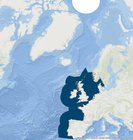
The magnitude of the CPUE over the six years is shown in Figure x. The radius of each circle is proportional to the CPUE value. Perhaps the most obvious conclusion from the maps is that there is considerable year-to-year variation in catches: 2015 is a low year; 2016 and 2017 are high years and 2020 is another low year.
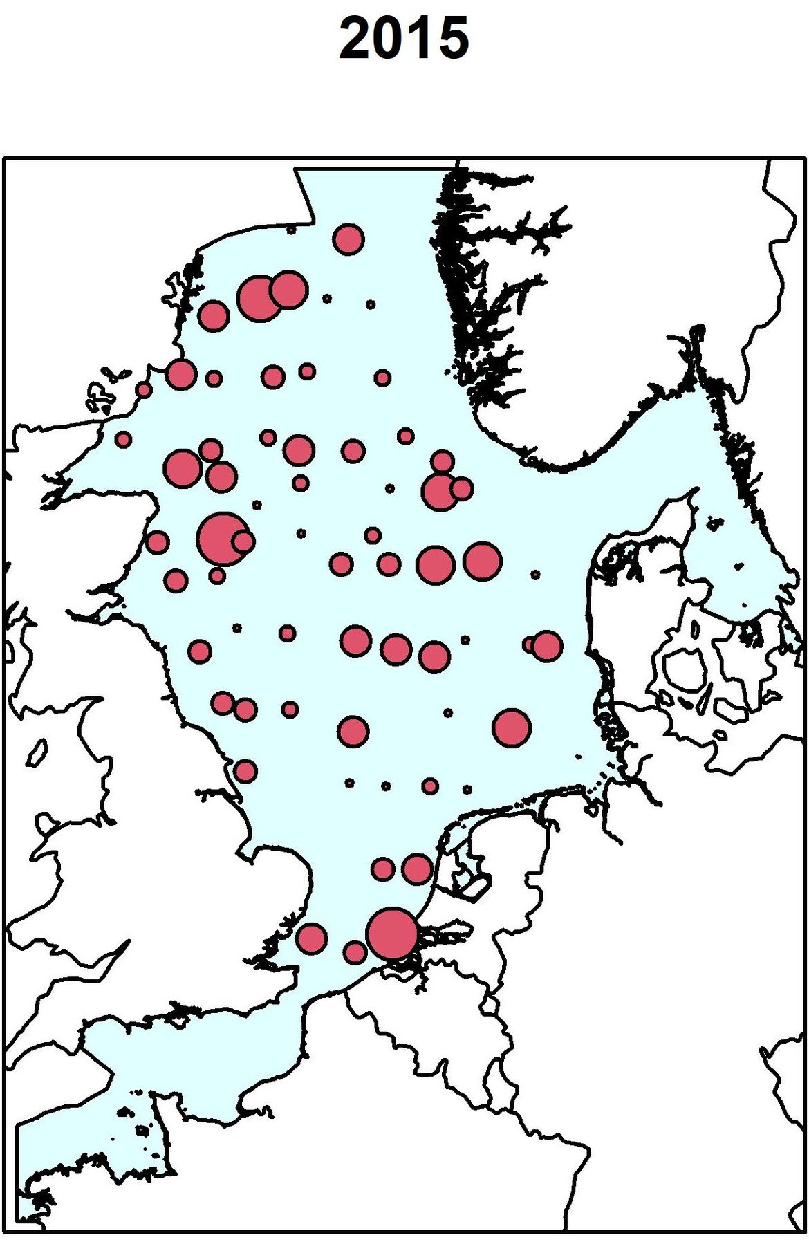
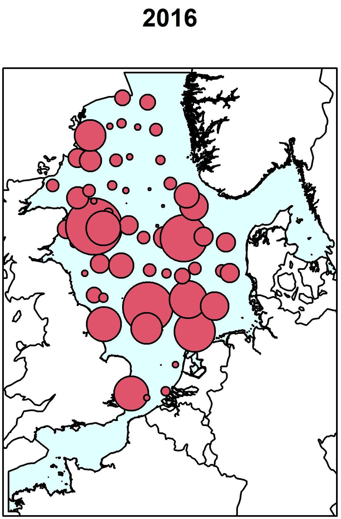
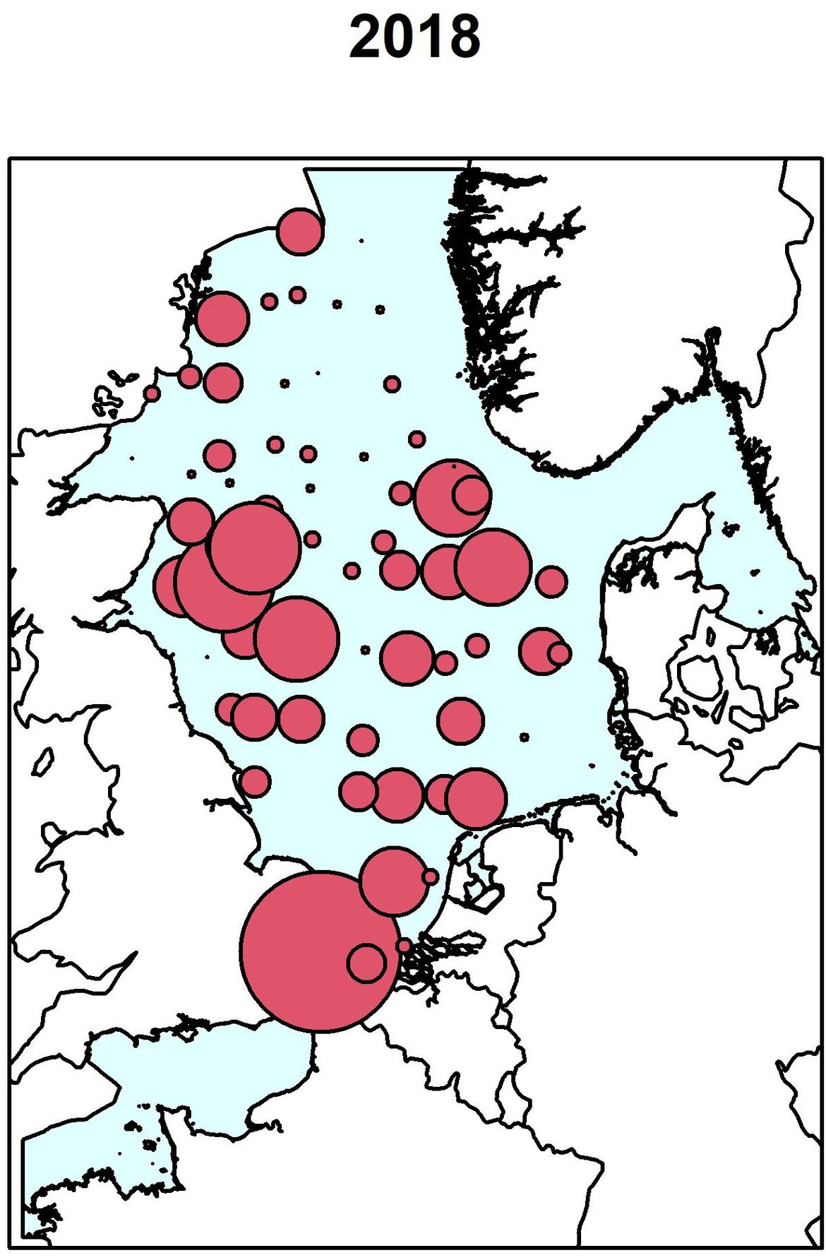
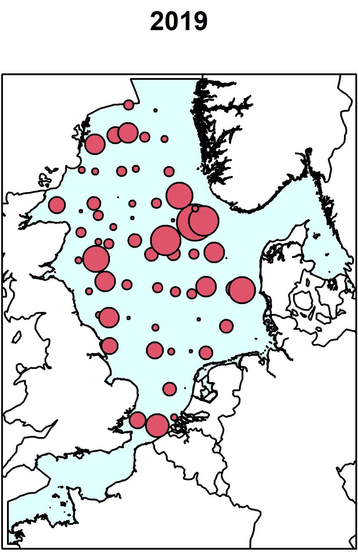
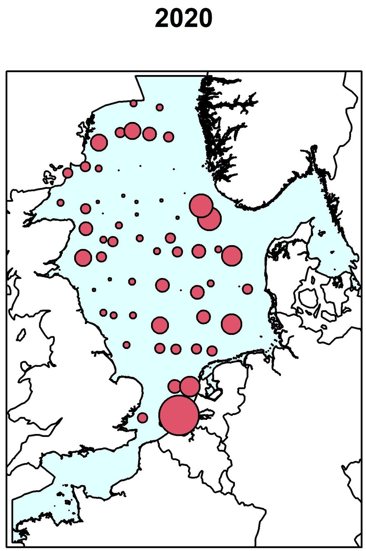
Figure x: Total litter counts for the UK NS-IBTS surveys between 2015 and 2020. The radius of each circle is proportional to the count at that point
Table m shows the mean levels of CPUE for each of the litter categories. Plastic and Fishing are the dominant categories.
| Litter | 2015 | 2016 | 2017 | 2018 | 2019 | 2020 |
|---|---|---|---|---|---|---|
| Plastic | 35 (33, 38) | 63 (58, 68) | 70 (65, 75) | 50 (45, 55) | 39 (37, 42) | 35 (32, 38) |
| Metal | 1 (1, 1) | 2 (1, 2) | 2 (2, 3) | 3 (2, 4) | 1 (1, 1) | 0 |
| Rubber | 1 (1, 2) | 3 (2, 3) | 1 (0, 1) | 4 (3, 5) | 3 (2, 4) | 1 (1, 1) |
| Glass | 0 | 0 | 0 | 1 (0, 1) | 2 (1, 2) | 0 |
| Natural | 1 (0, 1) | 3 (2, 5) | 0 | 1 (1, 2) | 3 (3, 4) | 1 (1, 1) |
| Fishing | 16 (15, 18) | 33 (30, 37) | 48 (43, 52) | 25 (22, 27) | 24 (22, 26) | 20 (18, 22) |
| Bags | 3 (3, 4) | 4 (3, 5) | 3 (2, 4) | 5 (4, 6) | 5 (4, 6) | 1 (1, 2) |
| Bottles | 0 | 0 | 0 | 1 (1, 2) | 0 | 1 (1, 2) |
To assess the spatial variation of the counts in each year, a GAM model was fitted, as described in the methods. Two obvious choices to model the counts are the Poisson and Negative Binomial distributions. It was assessed which might be best to use by fitting the probability density function for these distributions and comparing this to the smoothed empirical density function. The plots in Figure y suggest that the Negative Binomial is better as its fitted densities more closely correspond to the empirical densities. This was expected as litter is probably clustered, rather than distributed randomly over the seafloor.

Figure y: Comparison of Poisson and Negative Binomial probability densities to the smoothed, empirical distribution. The Negative Binomial is generally a closer fit to the empirical density
The Negative Binomial distribution was used for the GAM models. These models included both a spatial component (haul shoot latitudes and longitudes plus their interaction) and a term for area swept. The results showed that the spatial component was statistically significant only in 2017 and 2018. The resultant smoothed maps from these years are shown in Figure z. The 2017 map shows a south-east (high) to north-west (low) litter gradient. The 2018 map picks out the higher litter levels in the southerly part of the Region. However, these maps do not give much extra insight than that gained from the plots of the observed data in Figure x.
2017
2018
Figure z: Smoothed maps of UK NS-IBTS counts for 2017 and 2018 – the only two years that had a statistically significant spatial component. Available via https://odims.ospar.org/en/submissions/ospar_seabed_litter_counts_2017_09_001/ and https://odims.ospar.org/en/submissions/ospar_seabed_litter_counts_2018_09_001/
Demonstration study for catchability of litter materials by different gear types
Greater North Sea
Table n gives the Mean Of Ratio (MOR) values for each of the litter types. As expected, the MOR values for the lighter items, chiefly plastic, are less than those for the heavier items. This adds further credence to the theory that the GOV hauls are less efficient at collecting heavier items than the beam hauls.
| Litter type | Mean of the ratios of beam / GOV haul catch per km² |
|---|---|
| Total | 5,1 |
| Plastic | 4,4 |
| Metal | 8,3 |
| Rubber | 13,3 |
| Glass | 22,2 |
| Natural | 11,9 |
| Fishing | 4,0 |
| Bags | 5,1 |
| Bottles | 11,8 |
Celtic Seas
A similar method was used to calculate the ratio between beam and GOV hauls and between PORB and GOV hauls as was used for the Greater North Sea counts (although, this time, 90 squares were initially used, but most contained only one gear). However, as Figure j illustrates, there was limited scope to do this as there was a reduced spatial area where the gears overlapped.
In terms of the spatial squares used to capture places where both GOV and one of the other gears occurred, there were five for beam and GOV comparisons and three for PORB and GOV comparisons. Particularly, for the beam and GOV comparisons there was high variation between the ratios in the five squares. Thus, whilst the ratios give a guide as to the differences between the gears, it is recognised that their estimation is not precise.
Table o shows the estimated ratios for beam to GOV hauls and for PORB to GOV hauls for each litter item, where possible. There was insufficient data to calculate these ratios for some litter items. Clearly, the beam trawl hauls are much more efficient than GOV hauls. GOV and PORB hauls are more similar.
| Litter type | Mean of the ratios of beam / GOV haul catch per unit effort | Mean of the ratios of PORB / GOV haul catch per unit effort |
|---|---|---|
| Total | 12,2 | 1,2 |
| Plastic | 7,9 | 1,3 |
| Metal | 13,6 | 0,3 |
| Natural | 58,9 | - |
| Rubber | 8,1 | - |
| Glass | - | - |
| Fishing | 5,0 | 1,6 |
| Bags | 7,4 | 0,3 |
| Bottles | - | 0,9 |
Bay of Biscay and Iberian Coast
As for the analysis of proportions above, only BAK hauls above 40 degrees latitude and GOV hauls were used for counts. There has been previous work by Garcia-Alegre et al., (2020) on ratios between BAK and GOV hauls. This work needs to be considered for future assessments. However, for this preliminary analysis, the current data has been used to calculate BAK/GOV ratios for each of the litter categories. As can be seen in Figure o, there is limited scope to do this because there is only a small area in which GOV and BAK hauls are in proximity. However, data from this area has been used to calculate the ratios. These are shown in Table p.
| Litter type | Mean of the ratios of BAK / GOV haul catch per unit effort |
|---|---|
| Total | 0,91 |
| Plastic | 0,97 |
| Metal | 3,2 |
| Natural | 0,47 |
| Rubber | 0,71 |
| Glass | - |
| Fishing | 0,68 |
| Bags | 5,8 |
| Bottles | 5,4 |
Conclusion
Some broad conclusions can be drawn about the spatial and temporal changes in the chance that a haul contains litter in the Greater North Sea (GNS), Celtic Seas (CS), and Bay of Biscay (BB) and a demonstration study of count data in the Greater North Sea has been carried out. Plastic and fisheries related items are predominant in the top 10 using the probabilities for the three Regions and for the UK count case study. Catchability estimates can be given for the ratios between beam trawl and GOV, PORB and GOV, and BAK and GOV gears. To make further progress all surveys need to be giving reliable counts of litter items.
Modelling of the presence-absence data took into account potential biases caused by unequal sampling in space, area swept and gear type. However, it has been recognised that to be able to fully combine all the available data a better understanding and further detail about how the gears are set up, and how different countries have been interpreting the litter counting guidelines are required. The experience of fishing survey analyses should be drawn on to improve our modelling.
On the whole, there needs to be consideration about what seafloor litter data from fishing surveys demonstrates about the state of the seafloor and whether the data is useful for picking out spatial and temporal trends. There is moderate confidence in both the methodology and the data availability.
What we mean by the amount of litter on the seafloor needs to be defined. A working definition might be that this is the amount of litter within X cm of the sea bottom from below and Y cm from above. That is, the hauls might capture litter trapped in the sediment and floating just above the sea bottom.
Different fishing gears have different abilities to capture such litter. Beam trawls, for example, will be better at capturing litter in the sediment than GOV trawls. However, the two gears might capture similar amounts of litter above the bottom. Even beam trawls will probably not capture all the litter within a haul path.
It should be recognised that the haul data is almost certainly an under-estimate of the amount of litter on the seafloor. And different types of trawling gear will have different levels of bias (e.g., GOV trawls will have a bigger bias than beam trawls). But the important question is: “Does this matter?”.
The bias does matter if one is looking to know exactly how much litter is on the seafloor. Fishing surveys are not the most accurate way to determine the quantity of litter on the seafloor. A better method would be specialised surveys – perhaps involving dredging.
However, if one is interested in spatial and temporal trends then fishing surveys can provide useful information. Thus, even if the answers are biased, assuming the amount of litter caught in surveys is proportional to the true amount of litter on the seafloor and assuming fishing surveys with a specific net type performed comparably, then the fishing data can potentially provide good information on trends.
Some recent academic work on “zeros” in ecology has been done by Blasco-Moreno et al., (2019). These authors suggest that a zero-litter return from a haul is a “false zero” because the haul has missed litter that is present on the seafloor. However, as discussed above, these “false zeros” are simply an extreme version of the negative bias that we get from fishing hauls. They will affect any estimates of actual litter amount on the seafloor but should not affect estimates of trends.
There will, undoubtedly, be year-to-year changes in litter composition that are not due to some underlying trend. For example, there may be storm events or currents that expose litter more than at other times. Future work to better understand the impact climate change will have on marine litter is needed.
The year-to-year variation was clearly demonstrated by the study of counts from the NS-IBTS surveys – where there was confidence that counting practices were similar, that there were no changes to gear set-up and that similar areas were surveyed at the same time each year. However, even so, there were big year-to-year differences that were unable to be accounted for explicitly.
There needs to be a better understanding of the ‘life cycle’ of litter items when they reach the sea bottom. For example, items will get buried or decompose, they may be washed ashore or may disintegrate and become micro-litter. Understanding these life cycles will help to better untangle the data we see from the fishing surveys. For example, the data observed in 2020 may arise from 2020 but may also come from earlier years. Understanding the litter life cycle will help to estimate how much comes from previous points in time. There are several factors which influence the findings:
- The process and pathways involved for an item to become marine litter are unclear and time frames might include several years. Transboundary litter items from regions far outside Europe will also find their way into this region and complicate direct relationships (Van Loon et al., 2020).
- The process by which litter becomes trapped along the way or on the seafloor. For example, different litter types may take different times to go from the water column to the seafloor. These processes will differ regionally due to different conditions and processes which influence an item’s residence time. Biofouling plays an important role in the buoyancy process and will vary locally because of temperature, surrounding water conditions, and species availability. The different bottom structures and substrates will play an important role, not only in capturing and releasing litter items, but also in how that area is fished e.g., trawling gear.
- Most litter materials, e.g., plastic, metal, and glass, do not degrade easily and therefore there should be an accumulation of litter in our sea regions unless litter is removed/ relocated by currents or fishing.
- Tides and storms may redistribute litter throughout the year and thus move it from one area to another.
- Information on seafloor litter comes only from soft sediment areas (mud and sand) where bottom fishing is done. There is no data from rocky regions as these areas are not surveyed as the standard survey gears are not suitable for hard ground.
- Small items such as cigarette butts, bottle tops, or pieces of plastic sheeting will not be collected by the trawl so the number of these items will be under-estimated in the surveys.
In terms of how the litter assessments can be improved, there are many areas that have been considered through work in expert groups. There has been insufficient time to introduce them into this assessment. However, continued work is needed so that they can be evaluated and potentially used for future OSPAR assessments.
- Thoroughly research the fishing literature, and speak to fisheries scientists to better understand how they allow for the effects of haul types and changes in the make-up of gears over time.
- Rather than using all the different surveys, consider using only the best data for particular regions. That is, data where there is certainty that the counting of litter items has been consistent over a known period of time and where there are few changes in the way that fishing gear has been set up. It might be relevant to analyse beam trawl surveys more in depth as these seem to have a high MOR in relationship to GOVs. However, this would limit the spatial spread of data.
- Continue work in ICES WGML and OSPAR Seafloor Litter Expert group to ensure harmonisation of methods, specifically for counts so this data can be used for future assessments. New ICES technical guidelines will better define how to count litter items. It is vital the guidelines are shared with all Contracting Parties. With previous guidelines there was room for interpretation as to whether litter attached to the net was counted or not. Also, dolly rope fibres originating from the net itself are counted by some Contracting Parties but not all so this needs to be resolved.
- Look at whether there can be any relation to litter sources (urban areas, river inputs, fishing grounds, shipping lanes etc.) using the seafloor litter data.
- Decide what to do about very high count (e.g., one count is 1 100) or weight data. These will clearly influence modelling and estimation of summary statistics such as mean values. Experience from fishing surveys, where high counts are also observed, suggests that these data can be successfully modelled by zero-inflated models.
- As with our presence-absence modelling, the count data should be predicted or converted from different fishing gears to beam or GOV trawl data. But other standardising variables such as country and ship should be considered for all modelling.
- Evaluate the use of zero-inflated models to model count data.
- For GAM models, see whether area swept is better modelled by a non-linear smoother and whether maximum likelihood or restricted maximum likelihood are better estimation methods than cross-validation (used currently).
- Improve the count assessment by, if possible, taking account of any spatial correlations when calculating confidence intervals.
- Complete further work to develop theoretical approaches to generate measures of variability for the Top 10 lists. Using a Bayesian approach could form part of a more comprehensive approach to modelling Top 10 lists for the regions.
- Fishing surveys often revisit the same station each year. Potentially, this could result in these areas having less litter than other ‘non station’ areas. We need to investigate whether this is true and, if so, how our results can be modified to take account of this.
Knowledge Gaps
Numerous knowledge gaps listed below have been identified during this assessment. Further work to a better understanding of these is needed to enable future assessments to improve and for a better understanding of seafloor litter.
As data for more years become available, future assessments should aim to detect trends for litter counts. A power analysis would be beneficial to indicate how big a trend can be detected. It would be beneficial if differences between how contracting parties count litter items and whether they do count could be sorted out. This would allow count data to be used for the three OSPAR regions rather than just a UK case study. To build onto this, future assessments should also start to look at litter weights; however, this will require improved data from surveys.
The following points could improve future assessments:
- What is the ‘life cycle’ of litter on the seafloor. We need a better understanding of how hydrodynamics, geomorphology and human factors influence the geographical distribution of litter on the seafloor.
- How do different types of sediment impact the behaviour of the litter and how much litter gets collected by the trawl?
- How do seasonal patterns, weather and changes in currents affect the litter distribution?
- How do sources relate to litter densities?
- How is litter transported within, for example, the North Sea system? Is it transported to deeper areas and thus not sampled nor counted, transported to the north and out of the North Sea or is it kept within the North Sea alternating between the seafloor and the shores?
- A better understanding of the catchability of gears and conversion factors. Building on work for BAKA and GOV gear by Sánchez et al., (1994) looking at fish species and Garcia-Alegre et al., (2020). The different catchabilities of litter on the seafloor should be assessed in any way to strengthen quantitative statements.
- Whether it is possible to compare different fisheries surveys (relates to gear types and methodologies). Also, different depths (impact gear behaviour) and varying survey station design, e.g., random stratified or fixed position. Contracting Parties who use fixed positions may be more likely to have localised decrease in litter over time as a result.
- Understanding of fisheries assessments and how they account for variables such as gear type, area swept, haul, survey design etc.
- How much of the litter on the seafloor gets collected during trawls? Building on O’Donoghue and Van Hal (2018) estimate of 5%.
- Work on the assessment beyond the OSPAR area to enable comparisons. This would require a further examination of data and methodology discussions between regional sea organisations.
- Do areas with high/low commercial trawling intensities affect the distribution and amounts of litter on the seafloor? And do other fishing gears also have an effect?
- There is a need to consider other approaches to monitor seafloor litter. The current monitoring programme is value for money as it provides a lot of data as part of an existing monitoring programme, however as it is opportunistic there are limitations and evidence gaps. A better understanding of the seafloor environment, as a major sink of marine litter is still needed.
Bergmann, M. & Klages, M. (2012) Increase of litter at the Arctic deep-sea observatory HAUSGARTEN. Marine Pollution Bullitin. 64, 2734–2741.
Bingel, F., Avsar, D. & Uensal, M. (1987) A note on plastic materials in trawl catches in the north-eastern Mediterranean. Meeresfirsch. - Reports Mar. Res. 31, 3–4.
Blasco-Moreno, A., Perez-Casany, M., Puig, P., Morante, M., Castelles, E. (2019) What does a zero mean? Understanding false, random and structural zeros in ecology. Methods in Ecology and Evolution. 10, 949-59.
Carrothers, P. (1980) Estimation of Trawl Door Spread from Wing Spread. Journal of Northwest Atlantic Fishery Science. 1, 81-89.
Canals, M., Pham, C,K., Bergmann, M., Gutow, L., Hanke, G., Sebille, E., Angiolillo, M., Buhl-Mortensen, L., Cau, A., Ioakeimidis, C., Kammann, U., Lundsten, L., Papatheodorou, G., Purser, A., Sanchez-Vidal, A., Schulz, M., Vinci, M., Chiba, S., Galgani, F., Langenkämper, D. (2021) The quest for seafloor macrolitter: a critical review of background knowledge, current methods and future prospects. Environment Research Letters. 16(2), 023001.
Enrichetti, F., Domonguez, C., Toma, M., Bavestrello, G., Canese, S., Bo, M. (2021) Assessment and distribution of seafloor litter on the deep Ligurian continental shelf and shelf break (N V Mediterranean Sea). Marine Pollution Bulletin. 151, 110872.
Galgani, F., Burgeot, T., Bocquene, G., Vincent, F. (1995a) Distribution and abundance of debris on the continental shelf of the Bay of Biscay and in Seine Bay. Marine Pollution Bulletin. 30, 58–62.
Galgani, F., Jaunet, S., Campillo, A., Guenegen, X., His, E. (1995b) Distribution and abundance of debris on the continental shelf of the north-western Mediterranean Sea. Marine Pollution Bulletin. 30, 713–717
Galgani, F., Souplet, A., Cadiou, Y. (1996) Accumulation of debris on the deep sea floor off the French Mediterranean coast. Marine Ecology Series. 142, 225–234.
Galgani, F., Leaute, J.P., Moguedet, P., Souplet, A., Verin, Y., Carpentier, A., Goraguer, H., Latrouite, D., Andral, B., Cadiou, Y., Mahe, J. C. , J. C. Poulard, J. C., Nerisson, P. (2000) Litter on the sea floor along European coasts. Marine Pollution Bulletin. 40, 516–527.
Galgani, F., Hanke, G., Werner, S., Vrees, L. De. (2013) Marine litter within the European Marine Strategy Framework Directive. ICES Journal. Marine Science. 70, 1055–1064
Galil, B. S., Golik, A., Türkay, M. (1995) Litter at the bottom of the sea: A sea bed survey in the Eastern Mediterranean. Marine Pollution Bullitin. 30, 22–24
Garcia-Alegre, A., Gonzalez-nuevo, G., Velasco, F., Otero, P., Gago, J. (2020) Assessment between trawl gears baka and GOV for the study of seabed litter. Clean Atlantic Report. (unpublished).
ICES (2017) Manual of the IBTS North Eastern Atlantic Surveys. ICES. Series of ICES Survey Protocols SISP 15. 92 pp.
MSFD Technical subgroup on Marine Litter (2013) http://publications.jrc.ec.europa.eu/repository/bitstream/JRC83985/lb-na-26113-en-n.pdf
Kammann, U., Aust, MO, Lang, T. (2018) Marine Litter at the Seafloor – Abundance and composition in the North Sea and the Baltic Sea. Marine Pollution Bulletin. 127, 774-780.
Ioakeimidis, C., Zeri, C., Kaberi, H., Galatchi, M., Antoniadis, K., Streftaris, N., Galgani, F., Papathanassiou, E., Papatheodorou, G. (2014) A comparative study of marine litter on the seafloor of coastal areas in the Eastern Mediterranean and Black Seas. Marine Pollution Bulletin. 89, 296–304.
Maes, T., Barry, J., Leslie, H., Vethaak, A., Nicolaus, E., Law, R., Lyons, B., Martinez, R., Harley, B., Thain, J. (2018) Below the surface: Twenty- five years of seafloor litter monitoring in coastal seas of North West Europe (1992- 2017). Science of The Total Environment. 630, 790-798.
Manly, B, F, J., & Alberto, J, A, N. (2020) Randomization, Bootstrap and Monte Carlo Methods in Biology: 4th edition. CRC Press.
Miyake, H., Shibata, H. & Furushima, Y. (2011) Deep-sea litter study using deep-sea observation tools. Interdisciplinary Study Environmental Chemistry. 261–269.
Moriarty, M., Pedreschi, D., Stokes, D., Dransfeld, L. & Reid, D. G. (2016) Spatial and temporal analysis of litter in the Celtic Seas from Groundfish Survey data: Lessons for monitoring. Marine Pollution Bulletin. 103, 195–205.
O’Donoghue, A. & Van, Hal, R. (2018) Seafloor Litter Monitoring: International Bottom Trawl Survey 2018. Wageningen University Research Report C052/18.
Pham, C. K., Ramirez-Llodra E., Alt C. H. S., Amaro T., Bergmann M., Canals M., Company, J. A, Davies, J., Duineveld, G. Galgani, F., Howell, K. J., Huvenne, V. I., Isidro, E., Jones, D. O., Lastras, G., Morato, T., Gomes-Pereira, J. N., Purser, A., Stewart, H. Tojeira, I. Tabau, X. Rooij, D. V., Tyler, P. A. (2014) Marine litter distribution and density in European seas, from the shelves to deep basins. PLoS One. 9, 4.
Sánchez, F., Poulard, JC., & de la Gandara, F. (1994) Experiencias de calibración entre los artes de arrastre baka 44/60 y GOV 36/47 utilizados por los B/O cornide de Saavedra y Thalassa. Informes técnicos (Instituto Español de Oceanografía). 156, 3-48
Schlining, K., von Thun, S., Kuhnz, L., Schlining, B., Lundsten, L., Chaney, L., Connor, J. (2013) Debris in the deep: Using a 22-year video annotation database to survey marine litter in Monterey Canyon, central California, USA. Deep-sea Research. Part I Oceanographic Research Papers. 79, 96–105.
Spengler, A. & Costa, M. F. (2008) Methods applied in studies of benthic marine debris. Marine Pollution Bulletin. 56, 226–230.
Stefatos, A., Charalampakis, M., Papatheodorou, G. & Ferentinos, G. (1999) Marine debris on the seafloor of the Mediterranean Sea: Examples from two enclosed gulfs in western Greece. Marine Pollution Bulletin. 38, 389–393.
Van Loon, W., Hanke, G., Fleet, D., Werner, S., Barry, J., Strand, J., Eriksson, J., Galgani, F., Gräwe, D., Schulz, M., Vlachogianni, T., Press, M., Blidberg, E. and Walvoort, D. (2020) A European Threshold Value and Assessment Method for Macro Litter on Coastlines. EUR 30347 EN, Publications Office of the European Union, Luxembourg, 2020, ISBN 978-92-76-21444-1, doi:10.2760/54369, JRC121707
Watters, D. L., Yoklavich, M. M., Love, M. S. & Schroeder, D. M. (2010) Assessing marine debris in deep seafloor habitats off California. Marine Pollution Bulletin 60, 131–138.
Wood, S, N. (2017) Generalized Additive Models: An Introduction with R, second edition. CRC Press. 467.
Contributors
Lead authors: Jon Barry and Josie Russell
Supporting authors: Ralf van Hal, Willem van Loon, Katja Norén, Ulrike Kammann, Francois Galgani, Jesús Gago, Bavo Dewitte, Olivia Gerigny, Clara Lopes, Christopher Kim Pham, Sofia Garcia, Ricardo Sousa, Anna Rindorf
Supported by: OSPAR Seafloor Litter Expert Group, Intersessional Correspondence Group on Marine Litter and Contracting Parties, the data providers, Clean Atlantic project and ICES Working Group on Marine Litter
Citation
Barry, J., Russell, J., van Hal, R., van Loon, W.M.G.M., Norén, K., Kammann, U., Galgani, F., Gago, J., De Witte, B., Gerigny, O., Lopes, C., Pham, C. K., Garcia, S., Sousa, R., Rindorf, A. 2022. Composition and Spatial Distribution of Litter on the Seafloor. In: OSPAR, 2023: The 2023 Quality Status Report for the North-East Atlantic. OSPAR Commission, London.
| Assessment type | Indicator Assessment |
|---|---|
| Summary Results | https://odims.ospar.org/en/submissions/ospar_seabed_litter_msfd_2022_06/ |
| SDG Indicator | 14.1 By 2025, prevent and significantly reduce marine pollution of all kinds, in particular from land-based activities, including marine debris and nutrient pollution |
| Thematic Activity | Human Activities |
| Relevant OSPAR Documentation | OSPAR Agreement 2017-06 - CEMP Guidelines on Litter on the Seafloor |
| Date of publication | 2022-06-30 |
| Conditions applying to access and use | https://oap.ospar.org/en/data-policy/ |
| Data Snapshot | https://odims.ospar.org/en/submissions/ospar_seabed_litter_snapshot_2022_06_001/ |
| Data Results | https://odims.ospar.org/en/submissions/ospar_seabed_litter_data_results_2022_06_001/ |
| Data Source | https://datras.ices.dk/Data_products/Download/Download_Data_public.aspx |