

Recovery in the Population Abundance of Sensitive Fish Species
D1 - Biological Diversity
D1.2 - Population size
The decline in abundance of sensitive fish species has been halted in the Celtic Seas and Greater North Sea. However, significant recovery of populations is only apparent in the Celtic Seas.
Area Assessed
Printable Summary
Background
OSPAR’s strategic objective with respect to biodiversity and ecosystems is to halt and prevent further loss in biodiversity, protect and conserve ecosystems and to restore, where practicable, ecosystems, which have been adversely impacted by human activities.
There are three fish indicators assessed in the Intermediate Assessment 2017. This indicator addresses the extent of population recovery among sensitive species. Fish species with life history traits such as large ultimate body size, slow growth rate, large length and late-age-at-maturity, are particularly sensitive to additional sources of mortality, for example fishing mortality. Populations of such species are known to have declined markedly in abundance through the 20th century, a period of marked expansion in fishing activity across the area assessed. Recovery in population abundance among a significant fraction of these species is therefore needed.
This assessment is calculated using catch data from scientific groundfish surveys. These are standardized monitoring programmes that occur each year in the same period taking representative samples according to specific guidelines.
Life-history theory explains the evolution of species’ life-history traits under different mortality scenarios. Stable environments, with low disturbance mortality, support communities characterised by ‘K-type’ life-history traits (large body size, slow growth rate, late age and larger size at maturation, lower fecundity, etc.) while communities in regions of higher disturbance are more dominated by species with opposite ‘r-type’ traits (MacArthur and Wilson, 1967; May, 1976; Stearns, 1977, 1992; Roff, 1993; Huston, 1994; Reznick et al., 2002). Life-history theory predicts that heavily exploited fish communities (high disturbance mortality) should have fewer K-type and more r-type species. Elasmobranch species are generally characterised by K-type traits and many elasmobranch populations declined markedly during the 20th century (Frisk et al., 2001; Greenstreet and Hall, 1996; Walker and Hislop, 1998; Greenstreet et al., 1999a; Greenstreet and Rogers, 2000; van Strien et al., 2009). Teleost species with similar K-type life histories also declined (Philippart, 1998; Rijnsdorp et al., 1996). By the 1960s, average life-history trait composition among the demersal fish assemblage had become more r-type orientated (Jennings et al., 1999a; Greenstreet and Rogers, 2000, 2006; Greenstreet et al., 2012a), and in closely related pairs of species, the species with the more K-type life-history traits showed the greatest population decline at a time when fishing activity was high (Jennings et al., 1998). A species’ life-history trait composition provides an indication of its capacity to cope with additional mortality, and so determines its sensitivity to human activities that raise mortality rates above natural ambient levels. Species with K-type life-history traits are particularly sensitive to the additional mortality associated with fishing (Jennings et al., 1998; Gislason et al., 2008; Hobday et al., 2011; Le Quesne and Jennings, 2012).
Fishing activity is widespread across the assessment area and has been intense for a century or more (e.g. Rijnsdorp et al., 1996; Jennings et al., 1999b; Greenstreet et al., 1999b, 2009, 2011; Piet and Jennings, 2005; Shephard et al., 2011; Modica et al., 2014). As populations of fish species with K-type life-history traits across the region are likely to be in a depleted state, achieving acceptable status for these sensitive species will require population recovery. However, some species may be unable to sustain any level of fishing mortality, which means population recovery may not be possible for all sensitive species if any sort of sustainable fishing industry is to be maintained (Le Quesne and Jennings, 2012).
To support assessment of the status of fish communities under the European Union Marine Strategy Framework Directive (MSFD), Greenstreet et al. (2012b) developed a sensitivity metric that could be used to identify suites of sensitive fish species, among the species sampled by groundfish surveys operating across the geographic area to be assessed. Greenstreet et al. (2012b) proposed a trends based approach to setting assessment values related to population recovery for each sensitive species sampled by a survey and/or the halting of further population decline. A binomial distribution is then used to determine whether population recovery had occurred among a significant fraction of the suite of sensitive fish species sampled in any given survey.
Indicator Metric and Data Collection
Population abundance metrics were determined using data collected by 12 groundfish surveys carried out across two separate regions: the Greater North Sea and the Celtic Seas. Six survey data sets were available for analysis for each region (Table a).
| Region | Survey Acronym | Survey Period |
|---|---|---|
| Celtic Seas | CSEngBT3 | 1993 - 2015 |
| CSIreOT4 | 2003 - 2015 | |
| CSNIrOT1 | 1992 - 2015 | |
| CSNIrOT4 | 1992 - 2015 | |
| CSScoOT1 | 1985 - 2016 | |
| CSScoOT4 | 1995 - 2015 | |
| Greater North Sea | GNSEngBT3 | 1990 - 2015 |
| GNSFraOT4 | 1988 - 2015 | |
| GNSGerBT3 | 2002 - 2015 | |
| GNSIntOT1 | 1983 - 2016 | |
| GNSIntOT3 | 1998 - 2016 | |
| GNSNetBT3 | 1999 - 2015 |
Acronym convention: First 2–3 capitalised letters indicate the region (CS: Celtic Seas; GNS: Greater North Sea). Next capitalised and lowercase letters indicate the country involved (Fra: France; Eng: England; Ire: Republic of Ireland; NIr: Northern Ireland; Sco: Scotland; Ger: Germany; Int: International; Net: Netherlands). International refers to the two international bottom trawl surveys carried out in the North Sea under the International Council for the Exploration of the Sea (ICES). Next two capitalised letters indicate the type of survey (OT: otter trawl; BT: beam trawl). Final number indicates the season in which the survey is primarily undertaken (1: January–March; 3: July–September; 4: October–December).
Standard data collected on these surveys comprises numbers of each species of fish sampled in each trawl sample, measured to defined length categories (i.e. a fish with a recorded length of 14 cm would be between 14.00 cm and 14.99 cm in length). By dividing the species catch numbers-at-length by the area swept by the trawl on each sampling occasion, the catch data are converted to estimates of fish density-at-length, by species, at each sampling location in each year. Summing these trawl-sample species density-at-length estimates across all trawl samples collected within each sampling stratum in each year (e.g. ICES statistical rectangles), and dividing by the number of trawl samples within each stratum per year, gives an estimate of the density (of each species and length category) within each sampling stratum in each year. Summing these sample stratum density estimates across all sampling strata sampled in each year, and dividing by the number of strata sampled, provides estimates of the average density (N), of each species (s) and length category (l), in each year, across the whole area covered by the survey. Summing these density estimates (Ns,l / km2) across all length classes provides the required estimate of species population abundance density (Ns / km2) in each year for each survey.
Two different sensitivity metrics were used to identify species considered to be sensitive to fishing mortality. The Average Life-history Trait (ALHT) metric is the same as the metric developed by Greenstreet et al. (2012b). The ‘Proportion Failing to Spawn’ (PFS) is a new sensitivity metric developed to address flaws in the earlier metric identified by the ICES Working Group on the Ecosystem Effects of Fishing Activities (ICES, 2016). Development of the PFS metric is fully documented in a supporting paper (Greenstreet et al., 2017a). Analyses for both metrics are presented to demonstrate that assessment outcomes were not unduly affected by choice of sensitivity metric. Where choice of metric affects the assessment outcome, the principal assessment outcome should be based on the PFS metric. Both metrics rely on the availability of several life-history trait parameters for each species. For example, maximum recorded length (Lmax), von Bertalanffy ultimate body length or length infinity (Linf), von Bertalanffy growth term (K), length at maturity (Lmat), and age at maturity (Amat). Compilation of these parameters for all 485 species encountered across the 12 groundfish surveys in the North-East Atlantic, and where missing, the methods used to estimate them, are fully described in Greenstreet et al., 2017b.
For each survey, the number of sensitive species encountered was first established. However, almost by definition, these species are among the rarest in each surveyed community, so for many species the data available were too sparse to support meaningful assessment. Only species encountered on 50% or more of occasions that each survey was carried out were considered to have been sufficiently well sampled as to support formal assessment. In the overwhelming majority of cases, box plots comparing the sensitivity metric scores of species meeting and failing to meet this 50% criterion confirm that species deemed sufficiently well sampled as to support formal assessment were representative, in terms of their sensitivity metric scores (and hence life-history trait composition), of the full suite of sensitive species encountered by each survey (Figure a and Figure b). Thus, if recovery was observed in a significant fraction of the species capable of supporting formal assessment, the same might be expected among the species sampled too infrequently to support formal assessment.
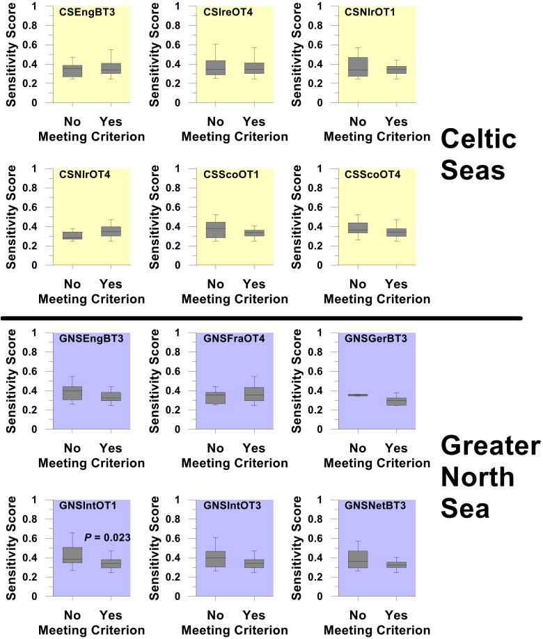
Figure a. Box plots comparing the Average Life-history Trait (ALHT) sensitivity metric scores of species sampled in each groundfish survey (see Table a for details of survey designation codes) that either met or failed to meet the ≥50% criterion
Box plots show the median sensitivity score (horizontal line), mid-50th percentile of scores (box) and range of score (whiskers). Where probability scores are shown, this indicates a statistically significant difference in sensitivity scores between those species capable of supporting formal assessment and those species failing to meet the ≥50% criterion.
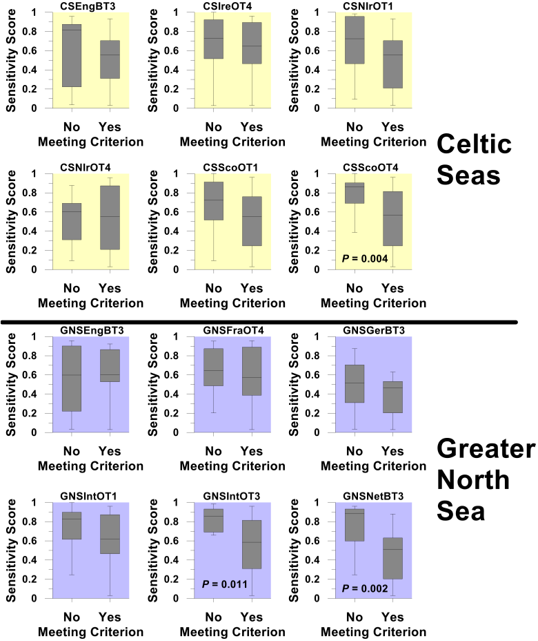
Figure b. Box plots comparing the Proportion Failing to Spawn (PFS) sensitivity metric scores of species sampled in each groundfish survey (see Table a for details of survey designation codes) that either met or failed to meet the ≥50% criterion
Box plots show the median sensitivity score (horizontal line), mid-50th percentile of scores (box) and range of score (whiskers). Where probability scores are shown, this indicates a statistically significant difference in sensitivity scores between those species capable of supporting formal assessment and those species failing to meet the ≥50% criterion.
Spatial Scope: Assessment Units
For each of the 12 groundfish surveys, population abundance density time-series were determined for all sensitive species, identified by either sensitivity metric, that were deemed capable of supporting formal assessment. Individual survey-based assessments were then performed. The individual survey-based assessments across the whole of the Celtic Seas and the Greater North Sea regions were then considered to determine overall assessment outcomes.
Baselines
None of the surveys extend sufficiently far back in time as to provide an adequate reference period to establish species abundance levels commensurate with acceptable status. A trends based assessment approach, relying on the use of trends based assessment values, was therefore adopted.
Assessment Values
By virtue of their sensitivity to additional human-related mortality, the population abundance of each sensitive species sampled by each survey is assumed to have declined as a result of past human activities. There is good evidence that fishing mortality has indeed caused declines in the populations of sensitive species.
Thus trends based assessment values related to population recovery constituted the primary basis for assessment; sensitive species should be increasing in abundance. However, should this primary assessment give an unacceptable outcome, or the results prove uncertain, a secondary assessment can be performed. The secondary assessment addresses an alternative question of whether further decline in the population abundance of sensitive species has at least been halted (Greenstreet et al., 2012b).
OSPAR Intermediate Assessment (IA) 2017 Indicator Assessment values are not to be considered as equivalent to proposed European Union (EU) Marine Strategy Framework Directive (MSFD) criteria threshold values, however they can be used for the purposes of their MSFD obligations by those Contracting Parties that wish to do so.
Primary Assessment: Recovery
Abundance trends for most species are not monotonic, so a simple parametric trends based approach (e.g. linear regression) is not appropriate; instead a non-parametric approach has been used. Essentially, the entirety of each survey time series acts as the reference period. The assessment value is set as: abundance in the assessment year must lie in the upper 25% of all abundance values observed throughout the time series.
For the purposes of the Intermediate Assessment (IA) 2017, the assessment year was the last year in each survey time series for which data were available. However, to explore recent trends, preceding years back to 2010 were also defined as the assessment year. The approximate period when data would have been available for the initial assessments required in 2012 under the European Union Marine Strategy Framework Directive (MSFD) was 2010. In assigning each consecutive preceding year as the assessment year, the length of the time series available to determine the upper 25% of all target abundance values diminishes. This places a limit on how far back in time the assessment can be pushed, particularly for surveys that only commenced more recently.
The surveys therefore provide abundance density estimates for each sensitive species in each year: a species-specific abundance metric for each sensitive species. These data can be ranked, and the ranking representing the lower boundary of the upper 25th percentile of all data for each species establishes the species-specific abundance metric-level assessment value for each species-specific abundance metric. In the stipulated assessment year, each species-specific abundance metric ranking should be greater than the ranking representing the species-specific abundance metric-level assessment value.
The sensitive species abundance indicator, for any given survey, is defined as the number of species in any assessment year whose species-specific abundance metric meets or exceeds its species-specific abundance metric-level assessment value. The metric meets or exceeds the assessment value when it is within the upper 25th percentile of all the abundance data over the whole survey time series, up to and including the year defined as the assessment year.
The sensitive species abundance indicator-level assessment value is defined based on probability. Random walk simulations suggest that the probability of the last abundance estimate datum in a time series falling into the upper 25th percentile of all data is 0.332. Knowing the number of assessed sensitive species in each survey, and the probability of any one species-specific abundance metric meeting its upper 25th percentile species-specific abundance metric-level assessment value, allows the sensitive species abundance indicator-level assessment value to be defined as the value that represents a significant (p<0.05) departure from the binomial distribution.
Secondary Assessment: Halt Further Decline
The logic underlying the alternative secondary assessment is identical to the logic described in relation to the primary assessment of population recovery objectives. The same simple non-parametric trends based approach can be used, except that in this instance, for each sensitive species in each survey, abundance in the assessment year must lie outside the lower 25% of all abundance values observed throughout the time series for the metric to meet its assessment value.
Following the same logic described for the primary assessment, the annual species-specific abundance metric data are ranked and the ranking representing the lower boundary of the upper 75th percentile of all data established as the new species-specific abundance metric-level assessment value; thus, in the stipulated assessment year, each species-specific abundance metric rank should be greater than the ranking representing the species-specific abundance metric-level assessment value.
The sensitive species abundance indicator, for any given survey, is defined as the number of species in any assessment year whose species-specific abundance metric meets or exceeds its species-specific abundance metric-level assessment value of being within the upper 75th percentile of all their own abundance data over the whole survey time series, up to and including the year defined as the assessment year. The random walk simulation suggest that the probability of the last abundance datum in a time series falling into the upper 25th percentile of all data is 0.332 for the primary assessment. Similarly, for the secondary assessment the probability of the last abundance datum in a time series falling into the lower 25th percentile of all data is also 0.332 and thus the probability of the last abundance datum in a time series falling into the upper 75th percentile of all data is 1 - 0.332 = 0.668. Following an identical logic to the recovery primary assessment, the number of assessed sensitive species and the probability of any one species-specific abundance metric meeting its upper 75th percentile metric-level target is known for surveys in the secondary assessment, allowing to define the sensitive species abundance indicator-level assessment value as the sensitive species abundance indicator value that represents a significant (at p<0.05) departure from the binomial distribution.
Assessment Integration Approaches
Two integration approaches, ‘probabilistic’ and ‘averaging’ were applied to determine integrated assessment outcomes at the regional scale.
Probabilistic Integration
Since the p<0.05 significance level, used to identify significant departures from a binomial distribution, is applied s the basis for setting sensitive species abundance indicator-level assessment values for each individual survey assessment, it follows that the probability of observing any one survey sensitive species abundance indicator actually meeting its sensitive species abundance indicator-level assessment value by chance is p≤0.05. Therefore the binomial distribution can again be used to determine the number of surveys where the indicator meets the indicator-level assessment value for a given number of individual survey assessments for this to represent a significant deviation from the binomial distribution. The probability of observing the sensitive species abundance indicator-level assessment value being met by chance is low. This results in the reliability of the probabilistic integration approach becoming questionable when the number of individual survey assessment outcomes that require integration becomes smaller.
Six survey assessment outcomes were available for both the Celtic Seas and Greater North Seas regions. This was considered to be just sufficient to allow for the use of the probabilistic integration method. Observing sensitive species abundance indicator-level assessment values met in two or more of the six surveys would represent a significant departure from the binomial distribution in both regions.
Averaging Integration
To apply an averaging integration approach, all survey sensitive species abundance indicator values were first converted to a Common-scale Indicator Score (CIS) by expressing sensitive species abundance indicator values as a fraction of their sensitive species indicator-level assessment values. Where individual indicator assessment values were met or exceeded the CIS was ≥1, where assessment values were not met the CIS was <1. These CIS values could then be averaged across all surveys carried out within each region to derive averaged integrated assessment outcomes. Where the averaged CIS was ≥1, the averaged integrated assessment outcome conferred acceptable status.
Results
The abundance of sensitive fish species is assessed against two different sets of assessment values. The first assessment examines whether population recovery is underway and the secondary assessment examines whether population decline has been halted. For the purposes of the Intermediate Assessment (IA) 2017, the assessment year was the last year in each survey time series for which data were available. Both assessments use two sensitivity metrics to define suites of sensitive species (Average Life-history Trait (ALHT) and Proportion Failing to Spawn (PFS)). Both metrics rely on species’ life trait information. Generally consistent results using either metric demonstrate that assessment outcomes were robust to choice of metric. However, the principal assessment outcome should be based on the more recently developed PFS metric.
Results were integrated across surveys within OSPAR regions to determine if the assessment values for recovery or halting decline were met using both ‘averaging’ and ‘probabilistic’ integrating procedures. Choice of integration procedure had minimal effect on assessment outcomes.
Here results for the assessments based on the PFS metric using the averaging integration method are presented. Population recovery among a significant number of sensitive fish species was evident in the Celtic Seas, but not in the North Sea (Figure 1). However in both regions, recent trends in the number of sensitive species increasing in abundance suggest an improving situation (Figure 2).
Further decline in the population abundance of sensitive fish species has been halted in both regions (Figure 3).
For this assessment the confidence in the methodology is moderate and the confidence in the data is high.
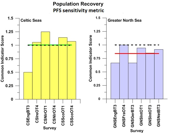
Figure 1: Outcomes against the ‘population recovery’ primary assessment for suites of sensitive species defined by the PFS sensitivity metric sampled by surveys carried out in the Celtic Seas and Greater North Sea
Outcomes for regional scale integrated assessments, using an averaging integration procedure are indicated by horizontal green line (meets or exceeds assessment value) or horizontal red line (does not meet assessment value), the assessment value is represented by a black dashed line. The Common Indicators Score is determined as indicator value / assessment value.
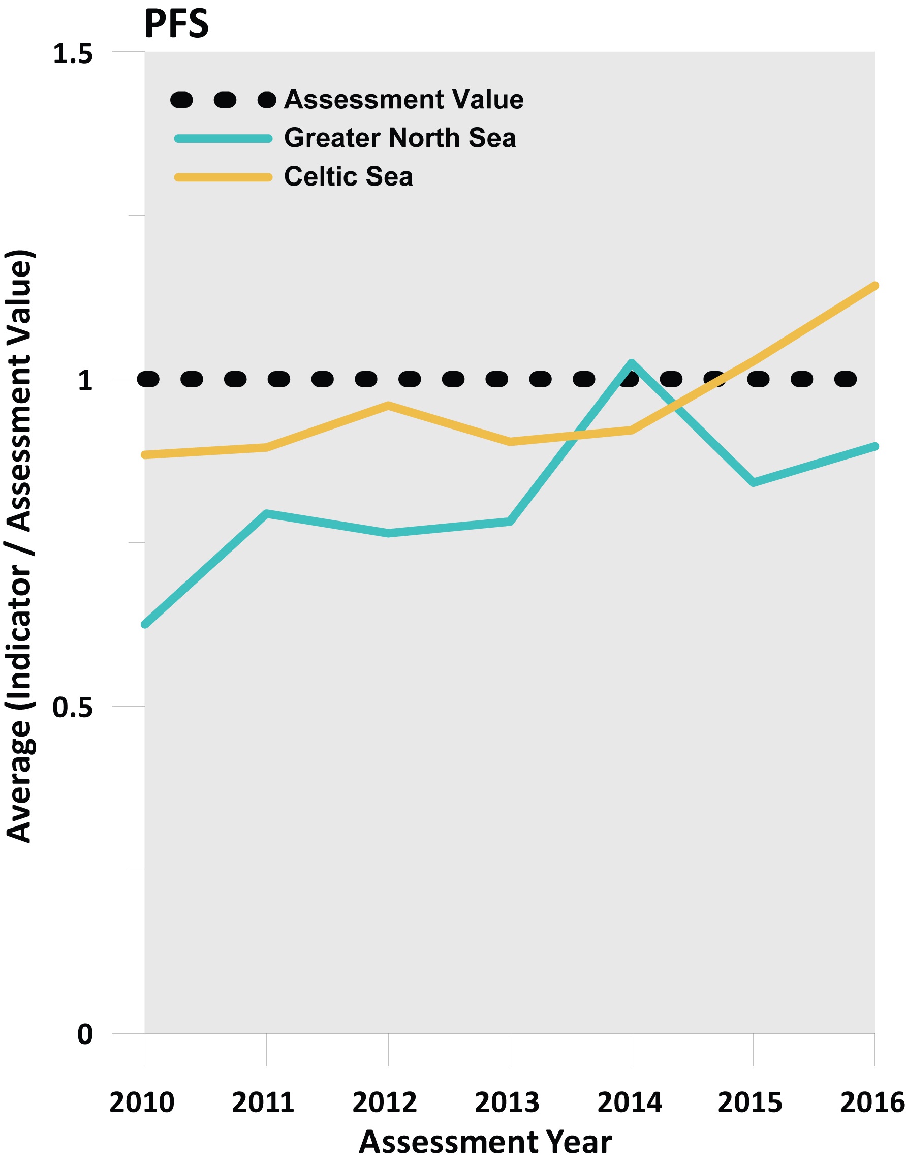
Figure 2: Integrated assessment outcomes for population abundance recovery (where a value above 1 means the assessment value is being met or exceeded) derived using an averaging integration approach
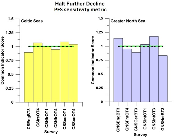
Figure 3: Outcomes against the ‘halt further population decline’ secondary assessment for suites of sensitive species defined by the PFS sensitivity metric sampled by surveys carried out in the Celtic Seas and Greater North Sea
Outcomes for regional scale integrated assessments, using an averaging integration procedure are indicated by horizontal green line (meets or exceeds assessment value) or horizontal red line (does not meet assessment value), the assessment value is represented by a black dashed line. The Common Indicators Score is determined as indicator value / assessment value.
This section presents the results of assessments using both sensitivity metrics to demonstrate that assessment outcomes were not affected by choice of sensitivity metric.
Primary Assessment: Assessment Values Related to Population Recovery
The sensitive species indicator-level assessment value was met in just one Greater North Sea survey regardless of the sensitivity metric used. In the Celtic Seas, the sensitive species indicator-level assessment value was met in four surveys using the Average Life-history Trait (ALHT) sensitivity metric, and in five surveys using the Proportion Failing to Spawn (PFS) sensitivity metric. Probabilistic integration was feasible for both the Celtic Seas and Greater North Sea regions where, with six surveys operating, seeing assessment values met in two or more surveys in each region represents a significant departure from the binomial distribution at p<0.05.
In the Celtic Seas region, the sensitive species indicator-level assessment value was met in four surveys using the ALHT sensitivity metric (Table b) and in five surveys using the PFS sensitivity metric (Table c). In both cases, the probability of these results occurring by chance was p<0.0001, so both probabilistic integrated assessment outcomes represented significant departures from the binomial distribution. In the Greater North Sea region the sensitive species abundance indicator met its sensitive species indicator-level assessment value in only one survey regardless of the sensitivity metric used (Table b and Table c), and this was not a significant departure from the binomial distribution for the integrated assessment outcome.
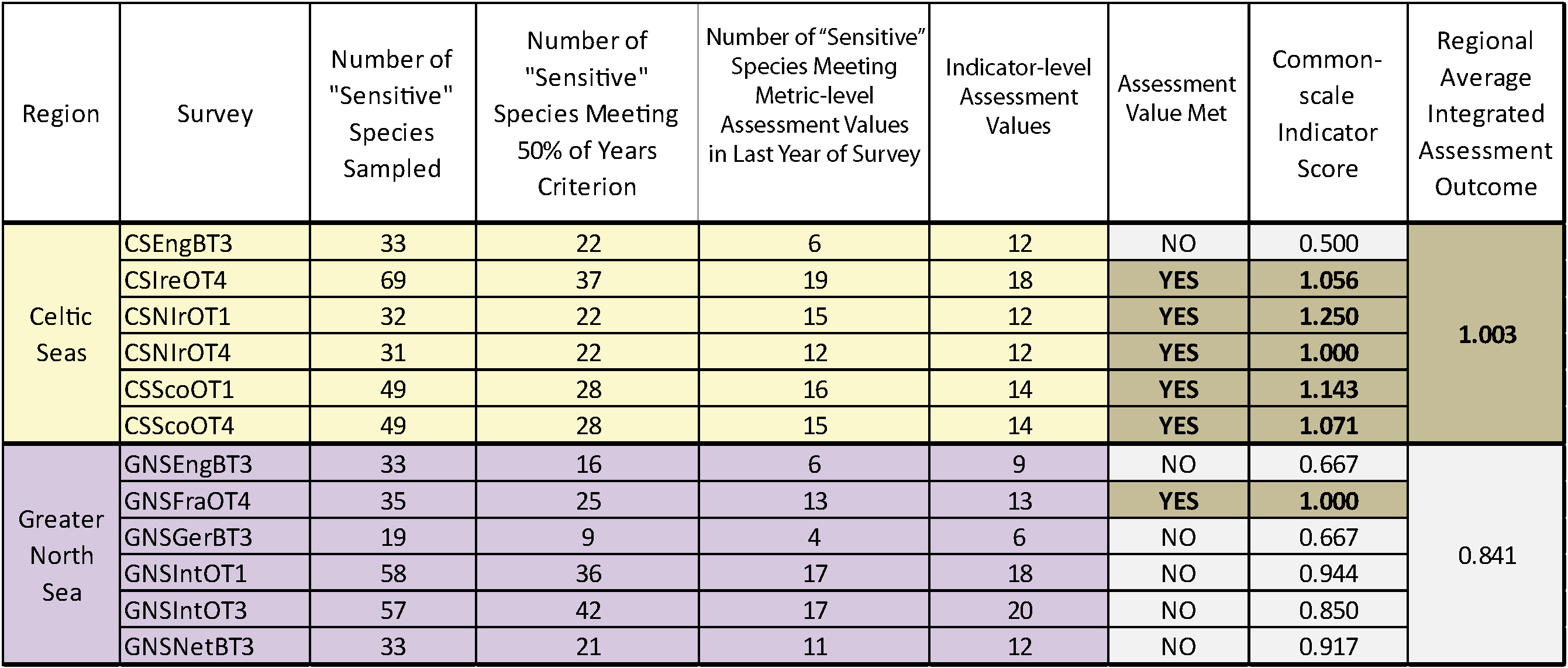
Table b. Assessment results based on using the ALHT sensitivity metric and probabilistic integration to define the suite of sensitive species in fish communities sampled by 12 groundfish surveys.
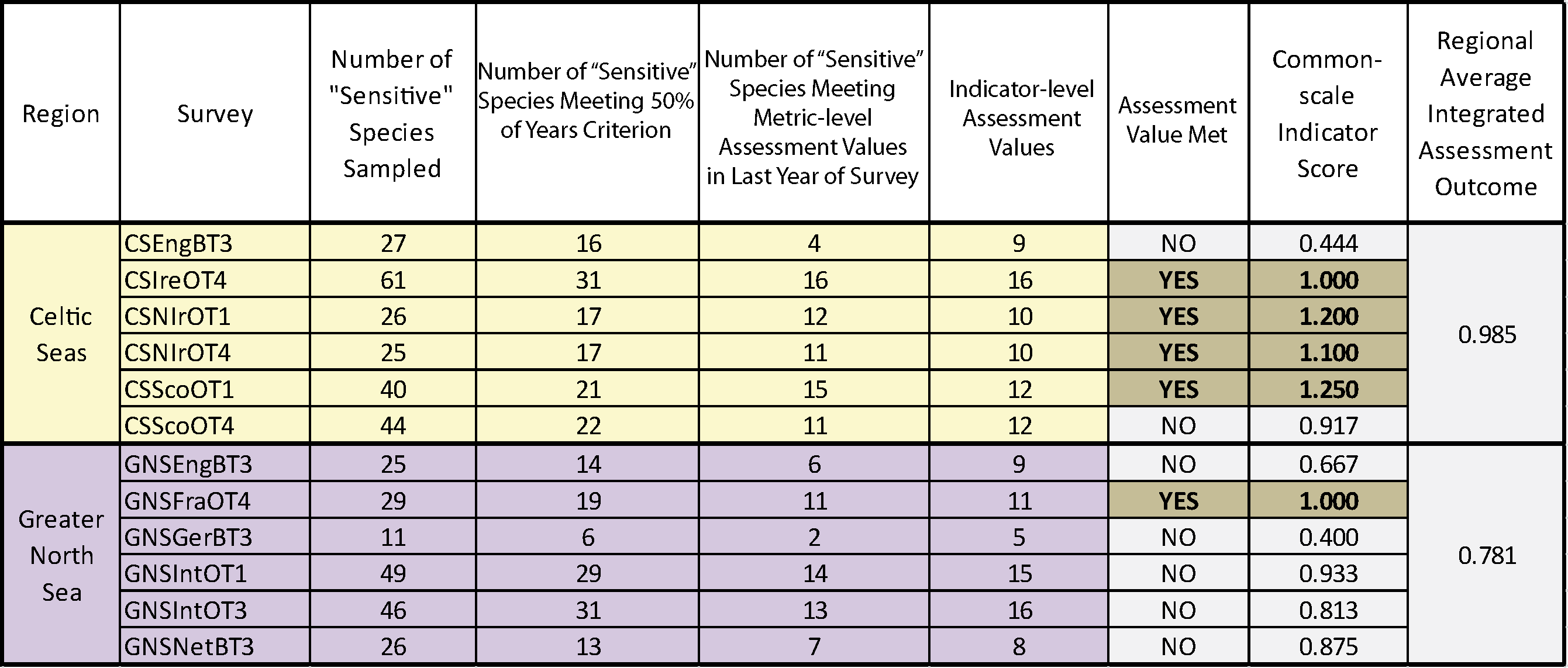
For each survey the table shows the number of sensitive species sampled, the number of these species meeting the 50% encounter rate criterion and so capable of supporting formal assessment, the sensitive species abundance indicator (i.e. the number of sensitive species for which their species-specific abundance metric meets or exceeds its population-recovery related species-specific abundance metric-level assessment value), and the species-specific abundance metric-level assessment value (i.e. the sensitive species abundance indicator value representing a significant (at p<0.05) departure from the binomial distribution), the individual survey assessment results (assessment value met – yes or no), the common-scale indicator score (i.e. indicator value / indicator assessment value) and the regional-scale average integrated assessment outcome (acceptable status if ≥1). Colour coding distinguishes surveys operating in different regions and assessment outcomes: Celtic Seas, yellow; Greater North Sea, purple.
Table c. Assessment results based on using the PFS sensitivity metric and probabilistic integration to define the suite of sensitive species in fish communities sampled by 12 groundfish surveys (for a full explanation of the columns please see the text for Table b).
Integrated assessment outcomes derived from the averaging integration were more conservative than the probabilistic integrated assessment outcomes. Again the integrated assessment gave an unacceptable outcome for the Greater North Sea regardless of the sensitivity metric used. But in this instance, the integrated assessment gave an acceptable outcome for the Celtic Seas only when using the preferred PFS sensitivity metric. When using the ALHT metric, the averaged integrated assessment outcome was unacceptable.
Trends derived from the two different sensitivity metrics were almost identical for any one survey. No trend or an increasing trend was observed more frequently for both metrics than a declining trend (Figure c and Figure d).
Although six surveys operated in both the Celtic Seas and the Greater North Sea regions, data were not available from all surveys in all assessment years from 2010 to 2016. Probabilistic integration was feasible in both regions for assessment years 2010 to 2015 when at least five surveys operated. In 2016, data were only available to support assessment from one Celtic Seas survey and two surveys in the Greater North Sea (Figure e). With so few surveys, obtaining an acceptable outcome would be extremely unlikely. Although the actual number of surveys operated in each year in each region varied, each individual survey-specific sensitive species abundance indicator value still had a probability of p=0.05 of meeting its sensitive species indicator-level assessment value in each year. Since the number of surveys generating data each year in each region was known, the binomial distribution could still be used to determine the number of surveys meeting the assessment value that would consitute a sgnificant departure from the binomial distribution at p<0.05.
Results were similar for the assessed years regardless of choice of sensitivity metric. In the Celtic Seas, the number of surveys where the sensitive species abundance indicator met its sensitive species indicator-level assessment value was significantly higher compared to what would be expected by chance in all years from 2010 to 2015 when based on the ALHT sensitivity metric, and in all years from 2011 to 2015 when based on the PFS sensitivity metric (Figure 1). Both metrics suggest an increasing trend in the fraction of surveys showing recovery in population abundance among a significant number of sensitive species. In the Greater North Sea, evidence has emerged only in more recent years of recovery in a significant number of sensitive species’ populations. For both metrics, and in both regions, the result was not significant in 2016, largely due to the small number of surveys (n=3) for which data were available (Figure e).
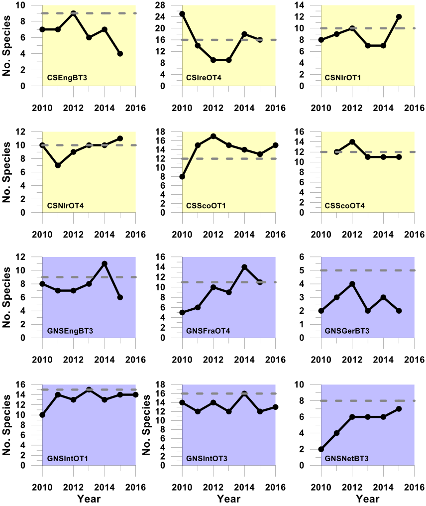
Figure c. Trends in the sensitive species abundance indicator against the primary recovery assessment using the ALHT sensitivity metric
Using the ALHT sensitivity metric to define sensitive species, these plots show, for each survey time-series, trends in the sensitive species abundance indicator (i.e. the number of sensitive species for which their species-specific abundance metric met or exceeded its recovery- related species-specific abundance metric-level assessment level (grey dashed line)) in successive assessment years from 2010 to the last datum. The ALHT sensitivity metric was used to define sensitive species. Colour coding distinguishes surveys operating in different regions: Celtic seas, yellow; Greater North Sea, purple.
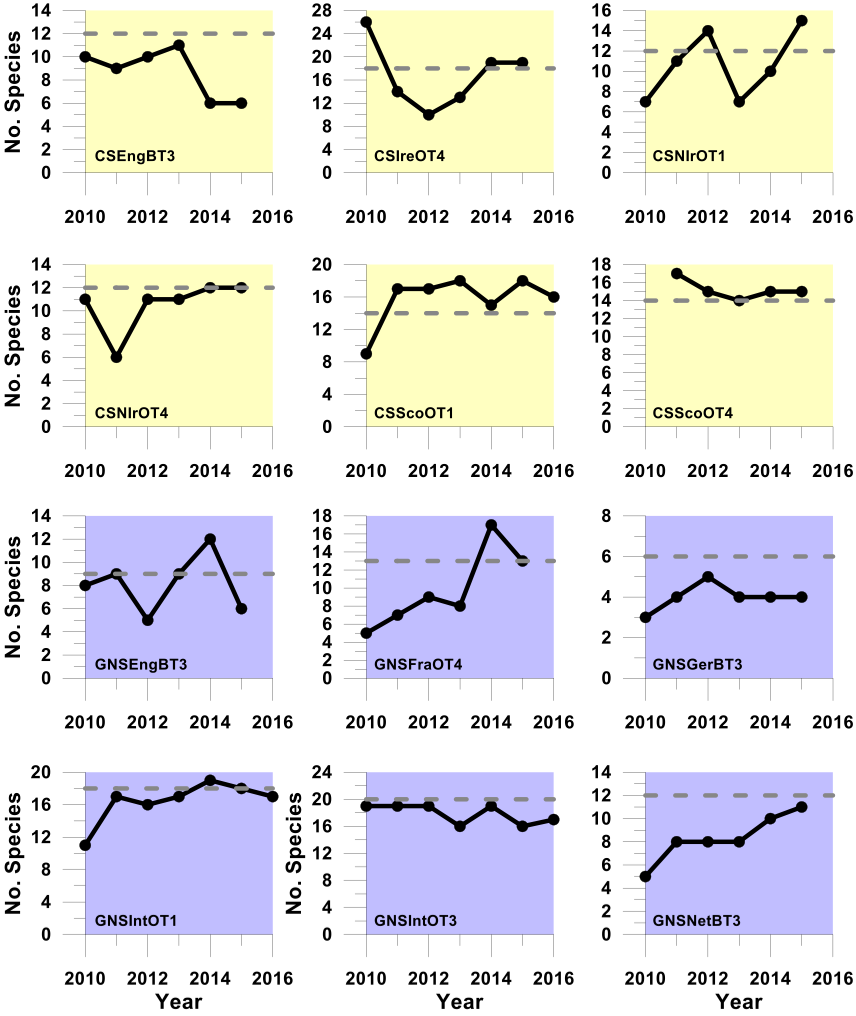
Figure d. Trends in the sensitive species abundance indicator against the primary recovery assessment using the PFS sensitivity metric
Using the PFS sensitivity metric to define sensitive species, these plots show trends in the sensitive species abundance indicator (i.e. the number of sensitive species for which their species-specific abundance metric met or exceeded its recovery-related species-specific abundance metric-level assessment value (grey dashed line)) in successive assessment years from 2010 to the last datum. Colour coding distinguishes surveys operating in different regions: Celtic seas, yellow; Greater North Sea, purple.
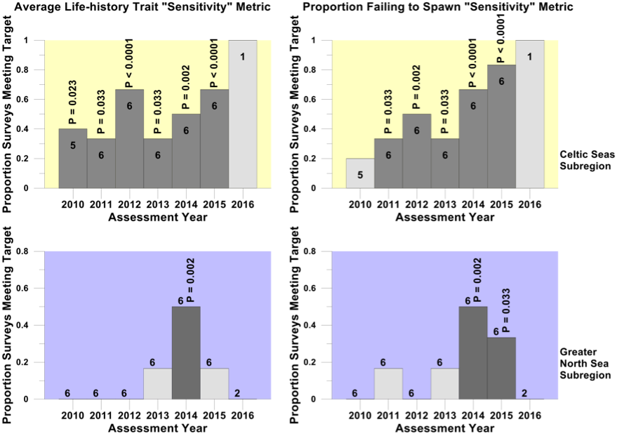
Figure e. Proportion of surveys where the sensitive species abundance indicator met the sensitive species indicator-level assessment value for the primary recovery assessment
Trends in the proportion of surveys in the Celtic Seas (yellow) and Greater North Sea (purple) regions where the sensitive species abundance indicator met its population-recovery related sensitive species indicator-level assessment value in each assessment year from 2010 to 2016. Numbers within each histogram bar indicate the number of surveys providing data for analysis. Light grey bars and dark grey bars indicate non-significant departures and significant departures respectively from the binomial distribution. The probabilities of observing each significant departure are shown above the histogram bars.
Use of an averaging integration method gave similar integrated assessment outcomes compared to the probabilistic integration method at the regional scale. The averaged integrated assessment value for recovery is achieved in the Celtic Seas region and not achieved in the Greater North Sea (Figure f).
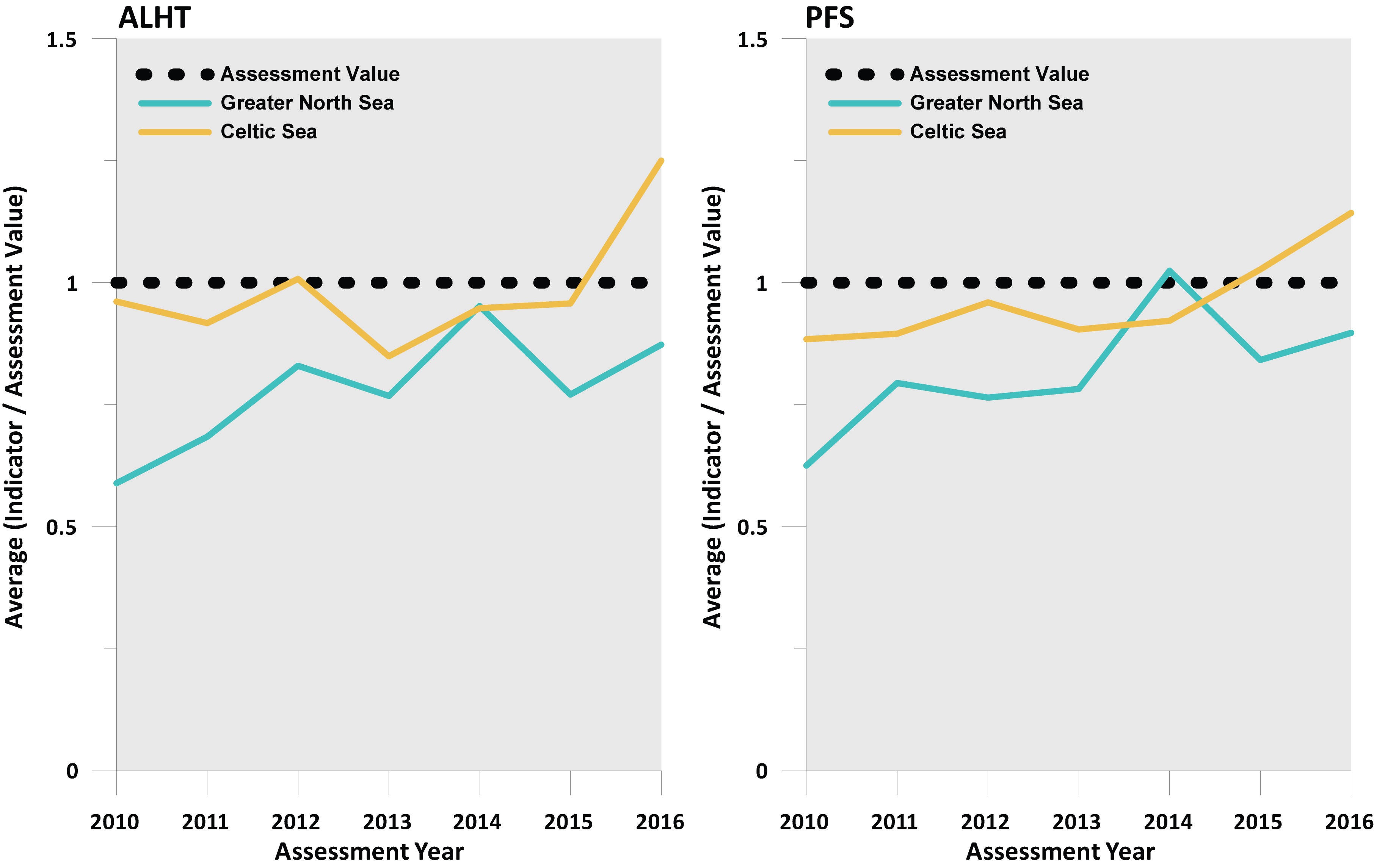
Figure f. Integrated assessment outcomes for population abundance recovery (where a value above 1 means the assessment value is being met or exceeded) derived using an averaging integration approach
The evidence supporting recovery among significant numbers of sensitive species in a significant number of surveys is uncertain. The regional scale integrated assessment outcome varied depending on the sensitivity metric used to identify the suite of sensitive species, and on the type of integration method used. There was more convincing evidence of recovery in the Celtic Seas compared to the Greater North Sea where evidence of recovery was scarce.
Secondary Assessment: Targets Related to Halting Further Population Decline
Rather than assessing against assessment values related to population recovery, an alternative secondary approach is instead to address the question as to whether current management regimes have at least halted further decline in the abundance of sensitive fish species. For this assessment, individual survey species-specific abundance metrics are required to lie inside the upper 75th percentile of all data observed throughout the time series. This represents the alternative species-specific abundance metric-level assessment value, and the probability of such an event occurring by chance is 0.668. As for the primary assessment, the actual sensitive species abundance indicator for any given survey is the number of species in any assessment year whose species-specific abundance metric meets or exceeds this alternative species-specific abundance metric-level assessment value. Knowing the probability of this happening by chance, the sensitive species abundance indicator-level assessment value can be defined as the sensitive species abundance indicator value that represents a significant (p<0.05) departure from the binomial distribution.
Regardless of the sensitivity metric used, probabilistic integrated assessment confirmed that further decline in sensitive species population abundance had been halted in both the Celtic Seas and Greater North Sea regions. In the Celtic Seas, sensitive species abundance indicator-level assessment values were met in four of the six surveys regardless of the sensitivity metric used; a highly significant departure from the binomial distribution at p<0.0001 (Table d and Table e). In the Greater North Sea, sensitive species abundance indicator-level assessment values were met in five surveys when the ALHT sensitivity metric was used (Table d), and in three surveys when the PFS metric was used (Table e). Both results represented significant departures from the binomial distribution at p<0.00012 and p<0.0022, respectively. An averaging integration approach gave slightly different results. When the PFS sensitivity was used, an acceptable assessment outcome was achieved in both regions (Table e), but when the ALHT sensitivity metric was used to identify sensitive species, the assessment outcome was not acceptable for the Greater North Sea. However, the sensitive species abundance indicator-level assessment value was missed by only a very small margin, primarily as a result of a single survey giving a poor assessment result (Table d). Trends for any one survey derived from the two different sensitivity metrics were almost identical (Figure g and Figure h).
Table d. Assessment results based on using the ALHT sensitivity metric and averaging integration to define the suite of sensitive species in fish communities sampled by 12 groundfish surveys (for a full explanation of the columns please see the text for Table b).
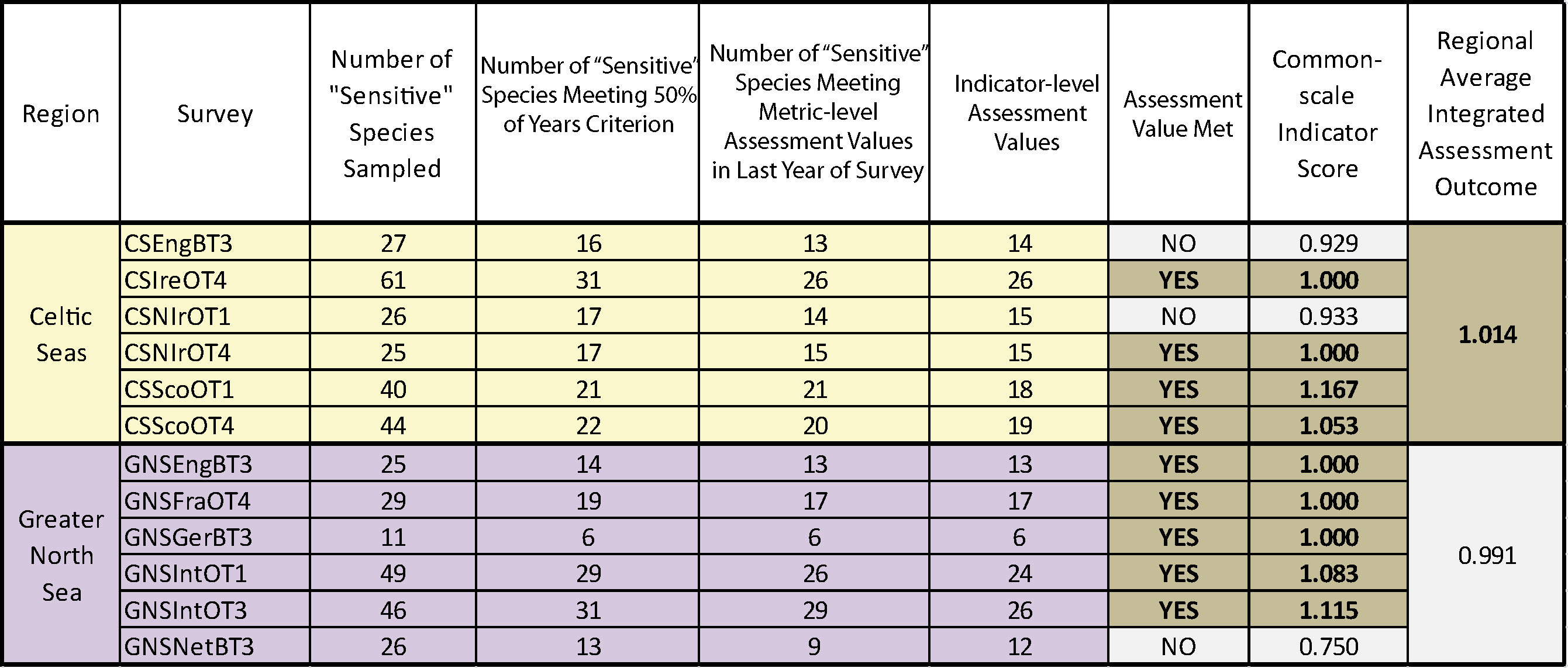
Table e. Assessment results based on using the PFS sensitivity metric and averaging integration to define the suite of sensitive species in fish communities sampled by 12 groundfish surveys (for a full explanation of the columns please see the text for Table b).
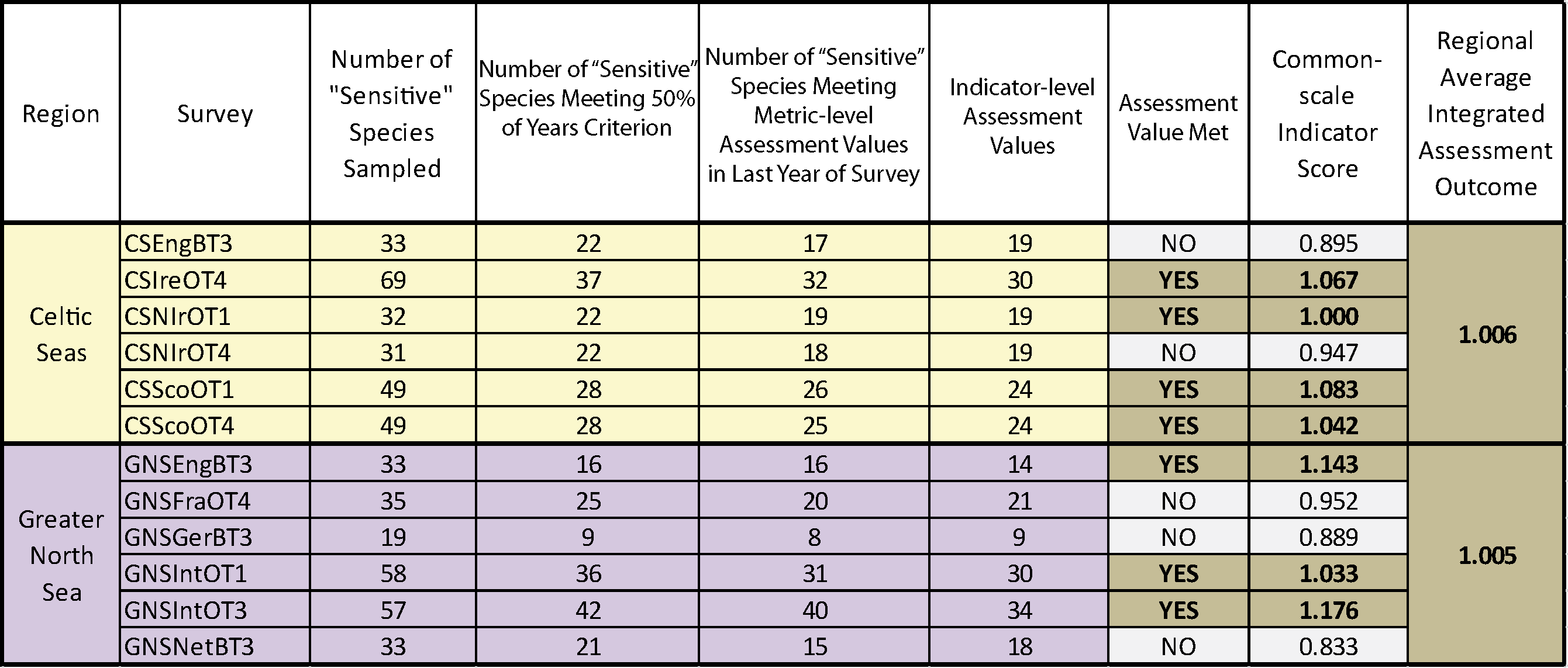
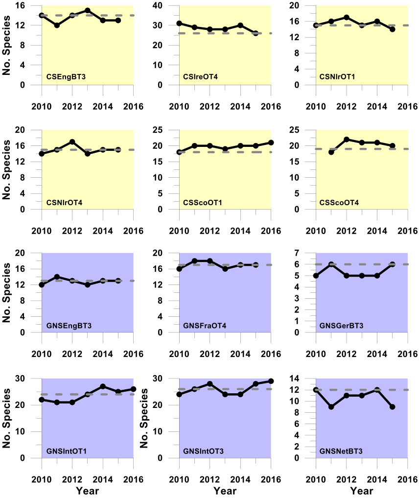
Figure g. Trends in the sensitive species abundance indicator against the secondary halting of further decline assessment using the ALHT sensitivity metric
Using the ALHT sensitivity metric to define sensitive species, these plots (Celtic Seas, yellow and Greater North Sea, purple) show trends in the sensitive species abundance indicator (i.e. the number of sensitive species for which their species-specific abundance metric met or exceeded its halt-further-population-decline related species-specific abundance metric-level assessment value (grey dashed line)) in successive assessment years from 2010 to the last datum. Colour coding distinguishes surveys operating in different regions: Celtic seas, yellow; Greater North Sea, purple.
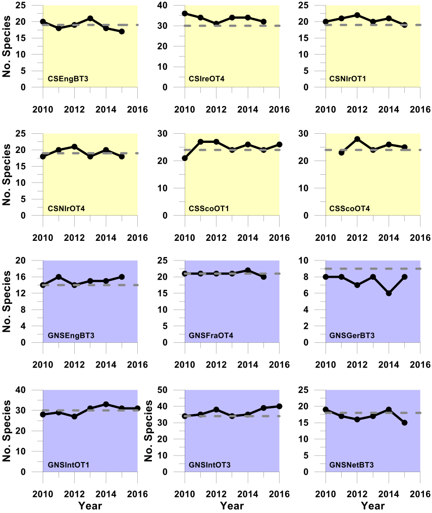
Figure h: Trends in the sensitive species abundance indicator against the secondary halting of further decline assessment using the PFS sensitivity metric
Using the PFS sensitivity metric to define sensitive species, these plots (Celtic Seas, yellow and Greater North Sea, purple) show trends in the sensitive species abundance indicator (i.e. the number of sensitive species for which their species-specific abundance metric met or exceeded its halt-further-population-decline related species-specific abundance metric-level assessment value (grey dashed line) in successive assessment years from 2010 to the last datum. Colour coding distinguishes surveys operating in different regions: Celtic seas, yellow; Greater North Sea, purple.
At the regional scale, sensitive species abundance indicator-level assessment values were achieved in a highly significant proportion of the six surveys operating in the Celtic Seas in all years since 2010, regardless of the sensitivity metric used, and in a highly significant fraction of the six surveys operating in the Greater North Sea in all years when the PFS sensitivity metric was used, and in all years except 2010 and 2013 when using the ALHT metric (Figure i). An averaged integrated assessment of individual survey assessments generally produced an acceptable status outcome in all years since 2010 at the regional scale. Averaged CIS values were around, or just above, the target value of CIS=1. Whenever a region trend dropped below a CIS value of 1, it did so by only the smallest of margins (Figure j).
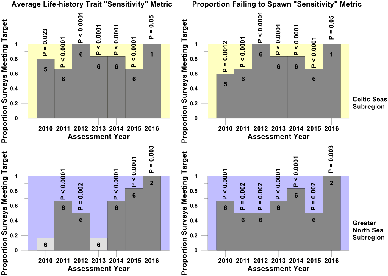
Figure i. Proportion of surveys where the sensitive species abundance indicator met the sensitive species indicator-level assessment value for the secondary halting further decline assessment
Trends in the proportion of surveys in the Celtic Seas (yellow) and Greater North Sea (purple) regions where the sensitive species abundance indicator met its halt-further-population-decline related sensitive species indicator-level assessment value in each assessment year from 2010 to 2016. Numbers within each histogram bar indicate the number of surveys providing data for analysis. Light grey bars and dark grey bars indicate non-significant departures and significant departures respectively from the binomial distribution. The probabilities of observing each significant departure are shown above the histogram bars.
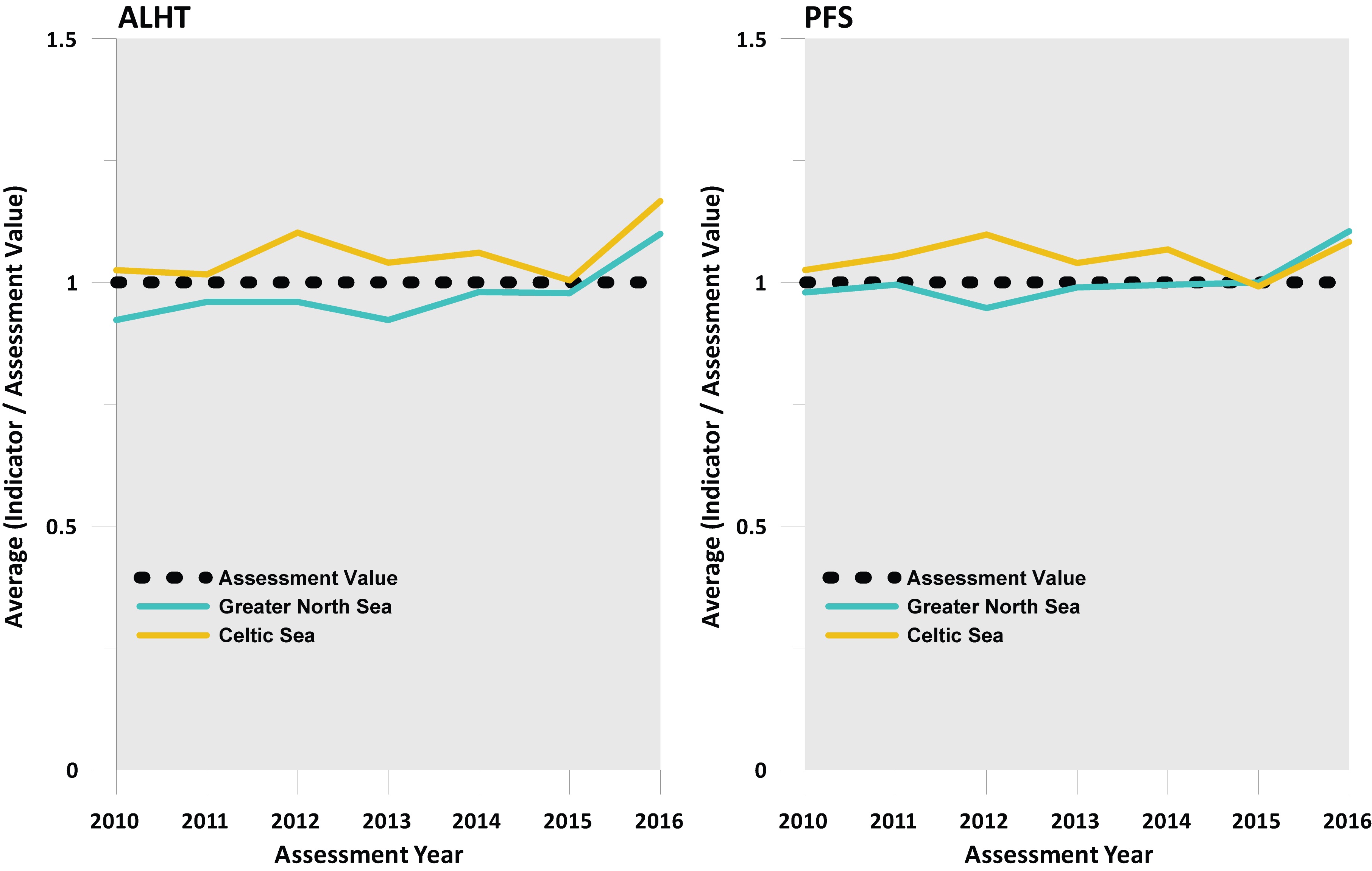
Figure j. Outcome of integrated assessment of whether population decline is halted (where a value above 1 means the assessment value is being met or exceeded) derived using an averaging integration approach
Summary of the assessment results
The information regarding the assessment (using the last datum in each survey time series) contained in Table b, Table c, Table d, and Table e is summarised in Figure k. This provides assessment results for each survey in each region, using both sensitivity metrics to define the suites of sensitive species, against both the primary assessment ‘population recovery’ and the secondary assessment ‘halt further population decline’, and based on the “averaging” integration procedure.
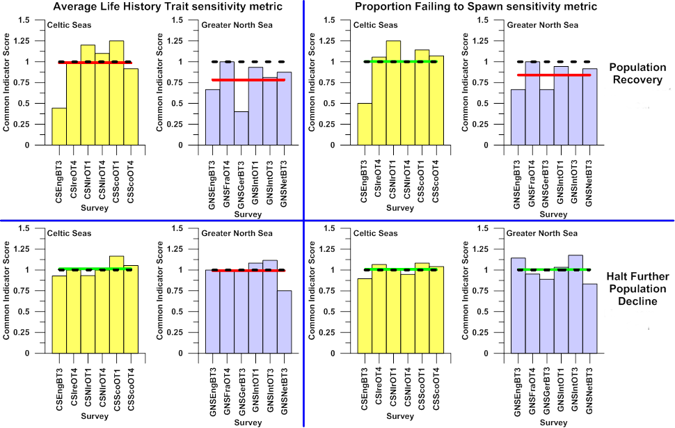
Figure k. Outcomes against both primary assessment ‘population recovery’ and secondary assessment ‘halt further population decline assessments for suites of sensitive species defined by both the ALHT and PFS sensitivity metrics sampled by surveys carried
Outcomes for regional scale integrated assessments, using an “averaging” integration procedure are indicated by horizontal green (meets or exceeds assessment value, represented by black dashed line) or red (does not meet assessment value) horizontal lines. The Common Indicators Score is determined as indicator value / assessment value.
Confidence Assessment
The majority of the assessment method has been published in peer-reviewed literature, however there are some new elements that have not. Therefore the confidence in the method is moderate.
There are no significant data gaps and there is sufficient spatial coverage therefore the confidence in the data is high.
Conclusion
When considering OSPAR regions individually, evidence of recovery was compelling in the Celtic Seas, but in the Greater North Sea the number of sensitive species increasing in abundance was insufficient to meet the assessment value.
Evidence to support a halt in decline of the abundance of fish species sensitive to fishing mortality is clear. Assessment outcomes suggested that decline has been halted since 2010. These conclusions are robust regardless of which sensitivity metric is used to define suites of sensitive species and the choice of integration method.
When considering all areas assessed (the Greater North Sea and the Celtic Seas), evidence to support the case that significant recovery had been achieved in the population abundance of sensitive species, was unclear. The assessment outcomes were influenced by which sensitivity metric was used to identify the suites of sensitive species in each survey, and also by the type of integration method applied to derive integrated assessment outcomes from the individual survey assessments.
Knowledge Gaps
The key knowledge gaps for the assessment are: the availability of suitable population dynamics models to support the setting of absolute abundance assessment values for sensitive fish species, the effects of warming seas on the scope for population growth and potential for population recovery among large-bodied sensitive fish species.
The lack of historical data precludes the use of absolute assessment values. The absence of survey data at times early enough to be considered suitable as reference periods precludes the use of an empirical approach to set assessment values for the absolute abundance of sensitive fish species, most of which are known to have become depleted well before the onset of any of the currently extant surveys. For the current assessment a trends based approach has been adopted, but this can only ever be a temporary stop-gap. Once such trends based assessment values are achieved, then the need for absolute abundance targets will become paramount because continuous increase in any species is biologically impossible. At some point each species’ population carrying capacity will be reached and resource limitation will cap any further population growth. In the absence of empirical data to support absolute abundance assessment value setting, populations dynamics models parameterised to represent specific fish communities could provide the only viable alternative. Part of the motivation behind the development of the PFS sensitivity metric is that the fraction of any cohort that actually survives to spawn at least once is a key variable in any population dynamics model.
A further knowledge gap relates to the effects of climate change on the potential for depleted sensitive species populations to recover. In many organisms, individuals in colder environments grow more slowly, but are larger as adults. This widespread pattern is embodied by two well-established rules: Bergmann’s rule, which describes the association between temperature and body size in natural environments, and which gives rise to gradients of increasing body size with latitude, and the temperature-size rule, which describes reaction norms relating temperature to body size in laboratory experiments (Anguilletta and Dunham, 2003). Large ultimate body size is a key life-history trait determining the ‘sensitivity’ of fish species to fishing mortality, and these temperature-size rules imply that warming seas might well inhibit population growth and reduce the potential for population recovery among large-bodied sensitive species.
Anguilletta M.J.Jr., Dunham, A.E. 2003. The temperature size rule in ectotherms: simple evolutionary explanations may not be general. American Naturalist, 162, 332-342.
Frisk, M.G., Miller, T.J., and Fogarty, M.J. 2001. Estimation and analysis of biological parameters in elasmobranch species: a comparative life-history study. Canadian Journal of Fisheries and Aquatic Sciences, 58: 969-981.
Gislason, H., Pope, J.G., Rice, J.C. and Daan, N. 2008. Coexistence in North Sea fish communities: implications for growth and natural mortality. ICES Journal of Marine Science, 65: 514-530.
Greenstreet, S.P.R., Fraser, H.M., Rogers, S.I., Trenkel, V.M., Simpson, S.D., and Pinnegar, J.K. 2012a. Redundancy in metrics describing the composition, structure, and functioning of the North Sea demersal fish community. ICES Journal of Marine Science, 69: 8–22.
Greenstreet, S.P.R. and Hall, S.J. 1996. Fishing and the ground-fish assemblage structure in the north-western North Sea: an analysis of long-term and spatial trends. Journal of Animal Ecology, 65: 577-598.
Greenstreet, S.P.R., Holland, G.J., Fraser, T.W.K., and Allen, V.J. 2009. Modelling demersal fishing effort based on landings and days absence from port, to generate indicators of “activity”. ICES Journal of Marine Science, 66: 886–901.
Greenstreet, S.P.R. and Rogers, S.I. 2000. Effects of fishing on non-target fish species. Effects of Fishing on Non-Target Species and Habitats: Biological, Conservation and Socio-economic Issues. (eds M. J. Kaiser and B. de Groot), pp. 217-234. Blackwell Science, Oxford, U.K.
Greenstreet, S.P.R. and Rogers, S.I. 2006. Indicators of the health of the fish community of the North Sea: identifying reference levels for an Ecosystem Approach to Management. ICES Journal of Marine Science, 63: 573-593.
Greenstreet, S.P.R., Rogers, S.I., Rice, J.C., Piet, G.J., Guirey, E.J., Fraser, H.M., and Fryer, R. J. 2011. Development of the EcoQO for the North Sea fish community. ICES Journal of Marine Science, 68: 1–11.
Greenstreet, S.P.R., Rossberg, A.G., Fox, C.J., Le Quesne, W.J.F., Blasdale, T., Boulcott, P., Mitchell, I., Millar, C., and Moffat, C.F. 2012b. Demersal fish biodiversity: species-level indicators and trends based targets for the Marine Strategy Framework Directive. ICES Journal of Marine Science, 69: 1789–1801.
Greenstreet, S.P.R., Spence, F.E. and McMillan, J.A. 1999a. Fishing effects in northeast Atlantic shelf seas: patterns in fishing effort, diversity and community structure. V. Changes in structure of the North Sea groundfish assemblage between 1925 and 1996. Fisheries Research, 40: 153-183.
Greenstreet, S.P.R., Spence, F.E., Shanks, A.M., and McMillan, J.A. 1999b. Fishing effects in Northeast Atlantic shelf seas: patterns in fishing effort, diversity and community structure. 2. Trends in fishing effort in the North Sea by UK registered vessels landing in Scotland. Fisheries Research, 40: 107–124.
Hobday, A.J., Smith, A.D.M., Stobutzki, I.C., Bulman, C., Daley, R., Dambacher, J.M., Deng, R.A., Dowdney, J., Fuller, M., Furlani, D., Griffiths, S.P., Johnson, D., Kenyon, R., Knuckey, I.A., Ling, S.D., Pitcher, R., Sainsbury, K.J., Sporcic, M., Smith, T., Turnbull, C., Walker, T.I., Wayte, S.E., Webb, H., Williams, A., Wise, B.S. and Zhou, S. 2011. Ecological risk assessment for the effects of fishing. Fisheries Research, 108: 372-384.
Huston, M.A. 1994. Biological diversity: the coexistence of species on changing landscapes. Cambridge University Press, Cambridge, UK
ICES. 2016. Report of the Working Group on the Ecosystem Effects of Fishing Activities (WGECO), 6–13 April 2016, Copenhagen, Denmark. ICES CM 2016/ACOM:25. 110 pp.
Jennings, S., Greenstreet, S.P.R. and Reynolds, J. 1999a. Structural change in an exploited fish community: a consequence of differential fishing effects on species with contrasting life histories. Journal of Animal Ecology, 68: 617-627.
Jennings, S., Alvsvíg, J., Cotter, A. J., Ehrich, S., Greenstreet, S.P.R., JarreTeichmann, A., Mergardt, N., Rijnsdorp, A.D. and Smedstad, O. 1999b. Fishing effects in Northeast Atlantic shelf seas: patterns in fishing effort, diversity and community structure. 3. International fishing effort in the North Sea: an analysis of spatial and temporal trends. Fisheries Research, 40: 125–134.
Jennings, S., Reynolds, J. D. and Mills, S. C. 1998. Life history correlates of responses to fisheries exploitation. Proceedings of the Royal Society of London, 265: 1-7.
Le Quesne, W.J.F. and Jennings, S., 2012. Predicting species vulnerability with minimal data to support rapid risk assessment of fishing impacts on biodiversity. Journal of Applied Ecology, 49: 20-28.
MacArthur, Robert H.; Wilson, E. O. 1967. The Theory of Island Biogeography. Princeton, New Jersey: Princeton University Press.
May, R. 1976. Theoretical Ecology: Principles and Applications. Blackwell Scientific Publishers. ISBN 0-632-00768-0
Modica, L., Velasco, F., Preciado, I., Soto, M., and Greenstreet, S.P.R. 2014. Development of the large fish indicator and associated target for a Northeast Atlantic fish community. ICES Journal of Marine Science, 71: 2403–2415.
Philippart, C.J.M. 1998. Long-term impact of bottom fisheries on several by-catch species of demersal fish and benthic invertebrates in the south-eastern North Sea. ICES Journal of Marine Science, 55: 342–352.
Piet, G. J., and Jennings, S. 2005. Response of potential fish community indicators to fishing. ICES Journal of Marine Science, 62: 214-225.
Reznick D., Bryant M. J., Bashey F. 2002r- and K-selection revisited: the role of population regulation in life history evolution. Ecology 83, 1509–152010.1890/0012-9658(2002)083[1509:RAKSRT]2.0.CO;2 (doi:10.1890/0012-9658(2002)083[1509:RAKSRT]2.0.CO;2
Rijnsdorp, A.D., Van Leeuwen, P.I., Daan, N., and Heessen, H.J.L. 1996. Changes in abundance of demersal fish species in the North Sea between 1906–1909 and 1990–1995. ICES Journal of Marine Science, 53: 1054–1062.
Roff, D. 1993. The Evolution of Life Histories. Chapman and Hall, New York. xii + 535 pp. ISBN: 0-412-02381-4, ISBN: 0-412-02391-1 (paper).
Shephard, S., Reid, D.G. and Greenstreet, S.P.R. 2011. Interpreting the large fish indicator for the Celtic Sea. ICES Journal of Marine Science, 68: 1963–1972.
Stearns, S.C., 1977 Evolution of life-history traits - critique of theory and a review of data. Annu. Rev. Ecol. Syst. 8: 145–171. doi: 10.1146/annurev.es.08.110177.001045
Stearns, S.C., 1992 The evolution of life histories. New York, NY: Oxford University Press
van Strien, A.J., van Duuren, L., Foppen, R.P.B. and Soldaat, L.L., 2009. A typology of indicators of biodiversity change as a tool to make better indicators. Ecological Indicators, 9: 1041-1048.
Walker, P.A. and Hislop, J.R.G. 1998. Sensitive skates or resilient rays? Spatial and temporal shifts in ray species composition in the central and north-western North Sea between 1930 and the present day. ICES Journal of Marine Science, 55: 392-402.
| Sheet reference | BDC17/D109 |
|---|---|
| Assessment type | Intermediate Assessment |
| Context (1) | Biological Diversity and Ecosystems - Targeted actions for the protection and conservation of species, habitats and ecosystem processes |
| Context (2) | OSPAR Publication 2009/406, EcoQOs on harbour and grey seal population trends |
| Context (3) | D1 - Biological Diversity |
| Context (4) | D1.2 - Population Size |
| Point of contact | OSPAR Secretariat |
secretariat@ospar.org | |
| Metadata date | 2017-09-15 |
| Title | Recovery in the Population Abundance of Sensitive Fish Species |
| Resource abstract | |
| Topic category | Environment |
| Indirect spatial reference | L1.2;L1.3 |
| N Lat | 62.0000000002998 |
| E Lon | 13.0665752428532 |
| S Lat | 48.0000507707265 |
| W Lon | -12.0250000001498 |
| Countries | |
| Date of publication | 2017-06-30 |
| Conditions applying to access and use | https://www.ospar.org/site/assets/files/1215/ospar_data_conditions_of_use.pdf |
| Data Snapshot | https://odims.ospar.org/documents/173/download |
| Data Results | https://odims.ospar.org/documents/175/download |