

Sentinels of the Seabed
Background
The attempts to implement an integrated ecosystem-based approach to manage anthropogenic activities and achieve a good environmental status of benthic habitats have been hampered by the lack of information on the condition of these habitats and their relationship with the pressures imposed. Anthropogenic disturbances produce changes to habitat condition, including modifications in species composition and their functions. Monitoring a group of keystone species (from a structural and functional point of view) provides useful insights into benthic habitat condition. Therefore, monitoring sentinel species (species characteristic of the habitat and sensitive to a given pressure) can provide a useful tool for knowing the habitat condition. The BH1 indicator aims to assess the environmental status using the proportional abundance of the sentinel species characteristics of this habitat across a pressure gradient. In this assessment, BH1 has been applied to generate specific pressure-state curves (which correlated the proportion of sentinel species with the level of trawling impact) for the evaluated Benthic Broad Habitats Types (BBHTs) under the MSFD. These curves have been applied to assess the impact of this pressure across these habitats, including determining areas highly disturbed by the pressure after defining a quality threshold for each BBHT.
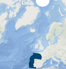
The Sentinels of Seabed (SoS-BH1, BH1 hereafter) indicator has been developed in the framework of the Benthic Habitats expert groups (OBHEG) of the Convention for the Protection of the Marine Environment of the North-East Atlantic (OSPAR) under the EU co-funded EcApRHA and NEA-PANACEA projects (Serrano et al., 2022, BH1 CEMP guidelines). This indicator is one of the five OSPAR standards developed to monitor and assess the benthic habitats' quality status within the OSPAR Maritime Area according to the Marine Strategy Framework Directive (MSFD; Directive 2008/ 56/E.C.); specifically, the BH1 is common for the assessment units Gulf of Biscay, North Iberian Atlantic, South Iberian Atlantic and Gulf of Cadiz (Figure a). The BH1 indicator was initially developed as BH1-typical species composition- following the OSPAR requirements and the corresponding criteria from the EU Commission Decision to achieve a Good Environmental Status (GES; 2010/77/EU). Afterwards, the indicator name was updated to its current form to better fulfil the requirements of the revised Decision to achieve GES (2017/848/EU; Serrano et al., 2022, CEMP guidelines document).
 and the area without bottom-trawling pressure (grey hatched area)")
Figure a: BH1 Common Indicator Assessment Units, the extent of the trawling footprint (bordered in red) and the area without bottom-trawling pressure (grey hatched area)
A benthic indicator is unlikely to be universally applicable since organisms are not equally sensitive to all types of anthropogenic disturbance (Buhl-Mortensen et al., 2009), geographical specifications (Dauvin, 2007) and habitat typologies (Tagliapietra et al., 2009). Keeping in mind these limitations common to all indicators, BH1 has been developed to approach as much as possible the characteristics of an ideal indicator (Hering et al., 2006) as it can detect changes in the community composition of marine habitats produced by any disturbance, physical or chemical if the species sensitivity to these disturbances is known. Specifically, BH1: (i) is adapted to each habitat by selecting a set of typical species from each habitat in areas with no pressure; and (ii) is responsive to any stressor type as long as there is an index available to evaluate species sensitivity to that pressure since these sensitivity indexes filter the previously selected typical species (e.g., BESITO index for trawling, González-Irusta et al., 2018). Nevertheless, as expected, the BH1 indicator is sensitive to data quality, which will dictate the power and utility of the resultant information.
Once the final set of sentinel species has been selected, changes in the proportion of these species across a pressure gradient can be computed to generate the pressure-state curves (Elliott et al., 2018). These curves are used in this assessment for two primary purposes: (i) to directly evaluate the status of habitat by transforming pressure units (e.g., swept area) into the proportion of sentinel species (using correlative models, e.g. GAMs), allowing to evaluate the status of the habitat across its extent (Figure b); (ii) to compute quality thresholds based on pressure state curves following the most recent recommendation of the EU Technical Group on Seabed Habitats (TGSEABED group) as well as previous works of OBHEG experts (Elliot et al., 2018). Finally, these values are converted into habitat status maps showing high, moderate, and low disturbance areas (Figure b) using quality thresholds previously computed based on the pressure-state curves (minimum proportion of sentinel species acceptable to keep ecosystem processes) specific for each habitat.
This document assessed the environmental status of BBHTs from the Gulf of Biscay, North Iberian Atlantic, South Iberian Atlantic and Gulf of Cadiz (using the BH1 indicator). The indicator has been applied from 2009 to 2021 following the OSPAR time range established for the Quality Status Report 2023 (QSR 2023), which has the objective of identifying and analysing information using long-term trends, but also from 2016 to 2020, the six-year period used by European Union (EU) Member States to assess progress from the second Article 8 reporting of the EU Marine Strategy Framework Directive (MSFD) in 2018, respectively.
This delivery is the first quantitative assessment of the extent of benthic habitats' quality status in response to bottom-trawling within the Common Indicator Assessment area (Figure a) using BH1, which allow to (i) establish the sensitivity of each habitat selected to the bottom-fishing activity, defining its environmental status across the pressure gradient and allowing the establishment of informed quality threshold following EU MSFD article 8 guidelines (European Commission, 2022); (ii) determine the extent of the habitat affected by trawling, predicting and mapping adversely affected areas and non-adversely affected areas. Therefore, the development of this indicator represents a substantial step forward in OSPAR's assessment capabilities within the Common Indicator Assessment Units -Gulf of Biscay, North Iberian Atlantic, South Iberian Atlantic and Gulf of Cadiz- for the QSR 2023.

Figure b: Interlinkage between data inputs, processes, and outputs for the BH1 indicator.
The methodology used to calculate the BH1 indicator to develop this assessment is briefly described below (for detailed information, see CEMP guidelines).
(i) Indicator inputs data and components
The BH1 uses three types of information: (i) the distribution of benthic habitats, (ii) the distribution and intensity of pressures that disturb these habitats and (iii) biological sampled data of the abundance (preferably biomass although also works with density) of benthic species from each habitat across a pressure gradient (including no pressure/low-pressure areas). These three sources of information are combined with sensitivity indexes, such as the BESITO index (González-Irusta et al., 2018) for trawling disturbance, to calculate the ecological status of a given benthic habitat and the evolution across the assessment periods (Figure b).
Regarding the confidence levels in the data, it is important to highlight that: (i) the quality of the biological data depends mainly on the sample collection and taxonomic expertise of the analysis and the quality control for each of the monitoring networks; and (ii) spatial and temporal resolutions between the three input types must be compatible. (e.g., good temporal agreement between the biological and pressure data).
The assessment based on the BH1 indicator has four main components, which are combined following the diagram in Figure b:
(i) A combined habitat map showing the distribution and extent of the BBHTs in the assessment unit (EMODnet, 2021)
(ii) A pressure map in a GIS format (raster format), such as trawling effort (ICES, 2021), showing the disturbance's distribution and extent that must be assessed.
(iii) Samples with biological information on species abundance across a pressure gradient within each BBHTs (e.g., data from IBTS with invertebrates abundances) to have data on the proportion of sentinel species at different levels of disturbance.
(iv) Response curves from statistical models which significantly correlate pressure values with sentinel species proportion (e.g., General Additive Models, GAMS).
(ii) Workflow of the assessment method
Step 1. Establishing habitat extent
The EUNIS (European Nature Information System) and its adaptation to the MSFD broad habitat is the classification used to implement this indicator. The indicator has been tested in both broad and special habitats (Serrano et al., 2022). The characteristics of special habitats and their often-high sensitivity to anthropogenic pressures prevents testing the indicator across the pressure gradient since the special habitat itself disappears and no samples remain at medium or high levels of pressure. Therefore, this assessment is focused on a selection of BBHTs based on them meeting two criteria: (i) they must be habitats submitted to trawling effort (i.e., it makes no sense to assess habitats that do not have bottom-fishing effort, e.g., depths shallower than 100 metres in the northern coast of Spain); (ii) they must have been biologically sampled with enough frequency to be included in the analysis (enough data to fit an informative pressure-state curve).
Step 2. Assessing the extent and distribution of pressures
The impacts on the seafloor associated with the bottom-contacting fishing activity are considered the most widespread disturbances in the OSPAR area. Therefore, this assessment only uses the fishing effort as a pressure. Trawling effort maps were derived using vessel GPS locations from the Vessel Monitoring Systems (VMS) and logbook data (gear information). Gear and GPS location data were linked using ship code and trip date fields. VMS pings unrelated to fishing activity were removed using speed and other criteria (ICES, 2021). To obtain the spatial distribution of swept area, hauls were assigned to individual fishing trips, and VMS pings were interpolated to obtain the fishing track of each haul using the cubic-hermite spline interpolation (Hintzen et al., 2010). The swept area was calculated by a c-square resolution (0,05˚) across the period analysed, the spatial resolution adopted by ICES (ICES, 2021). Since fishing pressure (SAR, swept area ratio) depended on the spatial resolution of the fishing pressure data (0,05° × 0,05° grid cells in this instance), the VMS data layers have conditioned the resolution of the BH1 assessment to that resolution.
ICES (2021) spatial data layers of fishing intensity used for this assessment were prepared by ICES in response to an OSPAR request within the OSPAR Maritime Area. However, the VMS data had some problems. VMS data from Portugal did not pass ICES quality checks, mainly due to the scarcity of data below 800 m of water depth. Therefore, some fleet activities may be absent or underrepresented, significantly affecting this evaluation. Problems were also found with the VMS data for Spanish waters compared with the most recent data facilitated by the Spanish Ministry of Agriculture, Food and Environment. VMS data from the North Iberian Atlantic assessment unit for the years between 2018 and 2020, as well as from the Gulf of Cadiz for all years, were underestimated. Although these Spanish problems have already been solved in the ICES database, the solution came after ICES released its advice (ICES, 2021). Therefore, for the assessment of Northern Iberia, the years from 2018 to 2020 have been discarded, and for the Gulf of Cadiz, the data provided by the Spanish Ministry of Agriculture, Food and Environment have been used.
The distribution of trawling effort (i.e., swept area ratio) map used to generate the geographical predictions of sentinel species proportion and the ecological status across the habitat, as will be explained later, was generated based on the mean values of fishing effort across the two assessment periods, (i.e., from 2009 to 2020 for QSR and from 2016 to 2020 for MSFD).
Step 3. Proportion of sentinel species determination
The BH1 indicator determines and analyses the proportion of a set of species identified as sentinel species across the trawling gradient to assess habitat sensitivity. The sentinel species are selected based on a double requirement: (i) species frequently found under reference conditions (typical species) and (ii) species sensitive to trawling (fragile species). To define frequent or typical species, two different metrics were applied: (i) intra-habitat similarity between stations sampled in the target habitat within reference conditions areas (no disturbance or very low disturbance) using the Similarity Percentages procedure (SIMPER; Clarke, 1993) and (ii) relative frequency for each species within the target habitat under reference conditions.
This set of frequent or typical species is filtered by prioritising species according to the BH1 sensitivity index (species responses to the analysed pressure), avoiding, when possible, tolerant species (i.e., those whose abundance does not show an apparent response to the pressure) and always avoiding opportunistic species (i.e., those whose abundance increases with the pressure). BH1 sensitivity index is calculated from available sensitivity classifications to a pressure or pressures group to select only typical and fragile species. This assessment used the BEnthic Sensitivity Index to Trawling Operations (BESITO, González-Irusta et al., 2018) for trawling disturbance, which scores species with values ranging from 1 to 5. Although these indexes are only applied for trawling, generating the list of sentinel species is the same and applicable to other pressures if species sensitive to the pressure are known. The method to generate the list of sentinel species has been compiled in a publicly available R function (https://github.com/Gonzalez-Irusta/SoS) which uses part of the code applied in Farriols et al., (2015) but adapted to the BH1 characteristics.
To establish the proportion of sentinel species, the biological samples (species abundance by haul) and the trawling effort associated with these samples (to establish the proportion of sentinel species across the pressure gradient) were used. The trawling effort was computed as the mean fishing effort of the four years prior to the sampling, including the year when the biological samples were taken. So, for instance, for the biological data sampled in 2013, the mean fishing effort of the period 2009-2013. Therefore, to assure consistency between available effort data (2009-2020) and biological data, the hauls distribution was analysed from 2013 to 2020 in the selected habitats. The hauls accomplished in each target habitat and areas with a swept area ration (SAR) ≤ 0,33 were used as a proxy to reference conditions to compute the typical species set. Afterwards, these typical species are filtered again based on their sensitivity to the pressure using the BESITO index (González-Irusta et al., 2018) to obtain the sentinel species (i.e., typical and fragile species) list for each habitat. The methodology for determining the sentinel species is described in detail in CEMP guidelines.
Once the list of sentinel species has been defined, its relative abundance (proportion) within each sampled value of disturbance is computed, and its evolution across the disturbance gradient is analysed to assess the habitat sensitivity.
Step 4. Assessing habitat response to the pressure: prediction of sentinel species
The correlation between the proportion of sentinel species and the trawling effort per habitat type was analysed using General Additive Models (GAMs), obtaining habitat response curves. Since the response variable was the proportion of sentinel species, they were analysed using a binomial GAM with Logit as a link function (Zuur et al., 2009). These pressure-state curves (as described in Elliot et al., 2018) were then applied to the trawling effort map (i.e., mean trawling effort across the assessment period) after masking them to the extent of each BBHTs extent polygons to generate a geographical prediction of sentinel species proportion across the habitat.
The BH1 is an empirical and risk-based indicator, but when no benthic sample data is available, it can be operated only as a risk-based indicator. In these cases, BH1 determines the response of BBHTs (where no benthic sample data is available) to pressure (trawling) through pressure-state curves for analogous BBHTs (well-sampled BBHTs, i.e., from nearby units of assessment).
Based on expert criteria, it was assumed that the BBHTs of the North Iberian Atlantic assessment unit respond to trawling similarly to the Gulf of Biscay and South Iberian Atlantic units (where there was a lack of data from benthic samples). Based on this assumption, the pressure-state curves of the well-sampled and analysed BBHTs in the North Iberian Atlantic unit are extrapolated to the similar BBHTs of these no-sampling units, where the trawling effort map of each unit is subsequently applied to generate the prediction of sentinel species proportion across the habitat. However, it is understood that, in spite of similarities, communities are different (especially in the northern part of the Gulf of Biscay) and that this may affect the response of these communities to trawling, generating differences with the equivalent habitats in the North Iberian Atlantic assessment. This has been directly acknowledged by assigning to these habitats a medium uncertainty.
Similarly, within the "well-sampled" units, there were BBHTs, specifically circalittoral habitats, where the lack of empirical data from the whole pressure gradient or the non-existence of reference areas in particular BBHTs prevented the empirical application of BH1. In these cases, it was assumed that the offshore circalittoral BBHTs respond similarly to the circalittoral MSFD habitats since they have similar environmental variables. Again, based on this assumption, the pressure-state curves of the well-sampled and analysed Offshore circalittoral MSFD habitats in these units were extrapolated to the circalittoral BBHTs to apply the pressure map subsequently and generate the prediction of sentinel species proportion across these habitats.
The analysis of the BBHTs using the BH1 indicator generates evaluations with different uncertainties, higher in cases where the extrapolation of curves is used and not curves generated based on accurate monitoring data. For this reason, the BH1 assessment contains the state maps of the BBHTs from the total Common Indicator Assessment area and the uncertainty maps associated with the state maps to consider this method's differentiation.
Step 5. Final assessment: habitat environmental status
Once the predicted values of sentinel species proportion across the habitat were generated, they were converted into high disturbance, moderate disturbance and low disturbance areas by using a quality threshold specific for each habitat (minimum proportion of sentinel species acceptable to keep ecosystem processes).
To establish the quality threshold for each habitat it was necessary to make three determinations based on the pressure-state curves of each habitat:
(i) Habitat sensitivity determination. The threshold must be defined based on the specific sensitivity of the habitats to guarantee the habitat quality. The habitat sensitivity was calculated by comparing the response curve for each habitat with five theoretical models using an R function developed for this purpose (see https://github.com/Gonzalez-Irusta/SoS). The theoretical models represent five possible responses to pressure, from a sensitivity of 1 (no sensitive) to 5 (very sensitive). The function assigns a value from 1 to 5 to each habitat based on the best fit between the theoretical model and the observed response to the pressure for that specific habitat (the lowest sum of squares of the differences between them). This calculation is repeated 1 000 times using bootstrapping on a dataset specific for each habitat (with only two columns, pressure and SoS values), obtaining the mean sensitivity of each habitat and its standard deviation based on the type of response observed in the BH1 indicator (see CEMP guidelines for a complete explanation). The mean sensitivity values are rounded to obtain the final integer value from 1 to 5.
(ii) Degradation point calculation. The method consists of identifying the point at which the habitat has lost most of its quality (degradation point) and establishing the quality thresholds at different distances to this point depending on its sensitivity, giving the most sensitive habitats the highest distance to degradation. The degradation point is the point at which the pressure-state curves change their trend, decreasing the rate at which the reduction in the habitat state is observed. Although several statistical tools are being explored to obtain this point, currently, the method relies on the 45 degrees slope of the tangent to the curve, previously used in different works to determine the tipping point in aggregation curves (Colloca et al., 2009; González-Irusta & Wright, 2017).
(iii) Quality thresholds definition. Once this point has been computed, the condition threshold is established as a percentile of the distance between the origin of the curve and the degradation point. The thresholds generated must respond to the range of sensitivities of the different habitats, so a more conservative one will be used for sensitive responses, while a more permissive one will be applied for habitats with more tolerance to the pressure. For that, three thresholds were defined: (i) the standard which corresponds with the middle point between the beginning of the curve and the tipping point (p.50), (ii) the precautionary located in the first third of that range (p.33) and (iii) the tolerant threshold (p.66).
This assessment used the precautionary threshold for habitats with a sensitivity value of 4, the standard for habitats with a sensitivity of 3 and the tolerant for habitats with a sensitivity of 2. The criteria that support the BH1 methodology for setting quality thresholds are the most appropriate to date, but it is temporary and may be modified in the future by expert agreements related to criteria to define the suitability of thresholds values.
Results
The present document assesses the level of disturbance of the main BBHTs affected by bottom trawling using the BH1 indicator in the common Indicator Assessment units: Gulf of Biscay, North Iberian Atlantic, South Iberian Atlantic and Gulf of Cadiz (Figure a).
The approach is fully quantitative, providing a map with continued values of the proportion of sentinel species for each evaluated BBHTs for the first time. These values are then converted into three disturbance categories using quality thresholds obtained from the pressure-state curves, providing values of low, moderate and high disturbance areas for both QSR (from 2009 to 2020) and MSFD (from 2016 to 2020) assessment periods (Figure 1, Figure 2).

Figure 1: Disturbance spatial distribution across the Common Indicator Assessment Units over the QSR time frame. Pie chart plots show the percentage of the assessment unit area under each disturbance level

Figure 2: Disturbance spatial distribution across the Common Indicator Assessment Units over the MSFD time frame. Pie chart plots show the percentage of the assessment unit area under each disturbance level
Total disturbance across the Common Indicator Assessment unit area:
- Disturbance occurred in 17.5% (QSR) and 16.9% (MSFD) of the total assessed area.
- In the QSR assessment, 6,78% of the evaluated area had high disturbance, 4,55% low and 4,22 moderate disturbances. In the MSFD assessment, 6.86% had high disturbance, 4,57% low and 3.67% moderate disturbances. Less than 2% of the disturbed area for both periods was not assessed due to the lack of biological data.
- The area with no bottom-trawling pressure covers 82,49% (QSR) and 83,10% (MSFD) of the total assessed extent.
Percentage of assessment unit area in each disturbance group:
- Bay of Biscay had the highest percentage of area with disturbance (QSR: 96,47%; MSFD: 96,07%), followed by the Gulf of Cadiz (QSR: 67,84%; MSFD: 64,14%).
- The Gulf of Cadiz presented the most significant percentage of area with high disturbance (QSR: 43,01%; MSFD:42,12%), followed by the Gulf of Biscay (QSR: 42,34%; MSFD: 40,81%).
- The highest percentage of areas with low disturbance occurred in South-Iberian Atlantic (QSR: 32,7%; MSFD: 28%), followed by North-Iberian Atlantic (QSR: 24,97%; MSFD: 22,85%).
- The highest percentage of areas with no bottom-trawling pressure occurred in South-Iberian Atlantic (QSR: 94,7%; MSFD: 95,58%), followed by North-Iberian Atlantic (QSR: 92,24 %; MSFD: 92,63%).
Habitat disturbance across all the common indicator assessment units:
- All the offshore and circalittoral BBHTs had areas with high disturbance.
- BBHTs with at least 50% of their area with high and moderate disturbance: offshore circalittoral coarse sediment, offshore circalittoral mixed sediment, offshore circalittoral mud, offshore circalittoral sand and circalittoral coarse sand.
- High disturbance was greatest in circalittoral coarse sediment (QSR: 64,56%; MSFD: 66,27%), offshore circalittoral mixed sediment (QSR: 57,87%; MSFD: 63,79%) and in offshore circalittoral mud (QSR: 42,77%; MSFD: 50,4%).
- Low disturbance was greatest in offshore circalittoral sand (QSR: 32,4%; MSFD: 34,86%) and upper bathyal sediment (QSR: 27,5%; MSFD: 25,23%).
- No trawling pressure was greatest in circalittoral mixed sediment (QSR: 79,93%; MSFD: 86,49%), circalittoral mud (QSR: 39,44%; MSFD: 41,07%) and upper bathyal sediment (QSR: 39,2%; MSFD: 44,32%).
Habitat disturbance within assessment units:
- The upper bathyal sediment and all the offshore and circalittoral MSFD broad habitats had areas with high or moderate disturbance for both periods, except for the South-Iberian Atlantic unit, in which circalittoral habitats and the offshore circalittoral coarse sediment had low disturbances.
- Offshore circalittoral mud had the largest or one of the most considerable proportions of high disturbance in all the assessment units except in the South Iberian Atlantic unit.
- One of the greatest low disturbance in assessment units was observed in the offshore circalittoral coarse sediment.
- The largest of one of the largest proportions of no trawling pressure was found in upper bathyal sediment.
The outcomes derived from assessing the environmental status of BBHTs from the units of assessment using the BH1 indicator are presented below.
The results will be presented for the agreed BH1 Common Indicator Assessment area (Figure a) to give an overview and be detailed for each of the four assessment units. In addition, the analyses and findings are presented across the two assessment periods: 2009 to 2020 and 2016 to 2020; the latter corresponds to the six years that Contracting Parties that are also EU Member States assess progress from the second EU MSFD Article 8 reporting in 2018.
(a) Habitat extent
(i) Overall Common Indicator Assessment area
The composite habitat map required to provide an overview of the extent and distribution of BBHTs from the Common Indicator Assessment area is shown in Figure c. This contextual information is completed with the data presented in Table a.
Table a: List of the BBHTs in the maritime waters of the Common Indicator Assessment area showing for each habitat the: area (km2), area trawled (km2), % of the habitat trawled and % of the trawling footprint which is represented in this habitat. The trawled area calculations have been determined by calculating the average SAR values for the two timeframes and SAR values > 0. Habitats that do not have at least 10% of their extent with no trawling pressure are highlighted in orange.
| MSFD BBHT | Area (km2) | Area trawling effort (km2) | % Habitat trawled | % Habitat total area trawled | BH1 Assessment | |||
| 2009-2020 | 2016-2020 | 2009-2020 | 2016-2020 | 2009-2020 | 2016-2020 | |||
| Off. Circa. Sand | 35106,48 | 33108,72 | 32886,58 | 94,31 | 93,68 | 24,63 | 25,36 | Assessed |
| Off. Circa. Mud | 31603,57 | 26124,50 | 25541,76 | 82,66 | 80,82 | 19,43 | 19,69 | Assessed |
| Upper Bathyal Sediment | 35982,27 | 21855,78 | 20010,48 | 60,74 | 55,61 | 16,26 | 15,43 | Assessed |
| Off. Circa. Coarse. Sediment | 11919,74 | 11566,14 | 11554,05 | 97,03 | 96,93 | 8,60 | 8,91 | Assessed |
| Circa. Sand | 16751,39 | 11315,71 | 11095,11 | 67,55 | 66,23 | 8,42 | 8,55 | Assessed |
| Circa. Coarse. Sediment | 8574,14 | 7987,39 | 7974,25 | 93,16 | 93,00 | 5,94 | 6,15 | Assessed |
| Off. Circa. Rock and Biogenic Reef | 7023,44 | 5529,47 | 5211,29 | 78,73 | 74,20 | 4,11 | 4,02 | Not Assessed |
| Circa. Mud | 6347,84 | 3847,96 | 3737,75 | 60,62 | 58,88 | 2,86 | 2,88 | Assessed |
| Upper Bathyal Sed/Rock -Biog. Reef | 1856,98 | 855,25 | 3100,64 | 46,06 | 39,17 | 0,64 | 0,56 | Not Assessed |
| Circa. Rock and Biogenic Reef | 7097,87 | 3079,65 | 2968,06 | 43,50 | 41,92 | 2,29 | 2,29 | Not Assessed |
| Off. Circa. Mixed Sediment | 3362,20 | 2879,47 | 2816,05 | 85,64 | 83,76 | 2,14 | 2,17 | Assessed |
| Upper Bathyal Rock and Biogenic Reef | 1856,98 | 855,25 | 727,39 | 46,06 | 29,17 | 0,64 | 0,56 | Not Assessed |
| Circa. Mixed Sediment | 2993,64 | 596,59 | 406,33 | 19,93 | 13,57 | 0,44 | 0,31 | Assessed |
| Infralittoral Sand | 2600,79 | 503,92 | 429,99 | 19,38 | 16,53 | 0,37 | 0,33 | Not Assessed |
| Infralittoral Rock and Biogenic Reef | 2041,74 | 483,32 | 455,93 | 23,67 | 22,33 | 0,36 | 0,35 | Not Assessed |
| Lower Bathyal Sediment | 12065,96 | 242,67 | 182,71 | 2,01 | 1,51 | 0,18 | 0,14 | Not Assessed |
| Infralittoral Coarse Sediment | 524,43 | 208,13 | 198,84 | 39,69 | 37,91 | 0,15 | 0,15 | Not Assessed |
| Infralittoral Mud | 767,05 | 190,18 | 142,61 | 24,79 | 18,59 | 0,14 | 0,11 | Not Assessed |
| Lower Bathyal Sed./Rock A | 35842,28 | 144,44 | 114,03 | 0,40 | 0,32 | 0,11 | 0,09 | Not Assessed |
| NA | 567,79 | 102,49 | 102,48 | 18,05 | 18,05 | 0,08 | 0,08 | Not Assessed |
| Infralittoral Mixed Sediment | 395,21 | 40,89 | 25,14 | 10,35 | 6,36 | 0,03 | 0,02 | Not Assessed |
| Lower Bathyal Rock-Biog. Reef | 493,87 | 6,15 | 3,74 | 1,25 | 0,76 | 0,00 | 0,00 | No Pressure |
| Upp- Bath. Sed/Low. Bath. Sed. | 6,88 | 5,91 | 5,91 | 85,84 | 85,84 | 0,00 | 0,00 | No Pressure |
| Upper Bathyal Rock and Biogenic Reef | 4,11 | 3,76 | 3,76 | 91,45 | 91,45 | 0,00 | 0,00 | No Pressure |
| Abyssal | 522215,5 | 1,57 | 1,57 | 0,00 | 0,00 | 0,00 | 0,00 | No Pressure |
| Total | 767541,4 | 134424,95 | 129696,45 | 17,51 | 16,90 | 100,00 | 100,00 | |
| % Area trawled assessed by BH1 | 88,74 // 89,46 | |||||||
| % Area trawled assessed, excluding trawling on rock habitats | 98,92 // 99,06 | |||||||
")
Figure c: Extent and distribution of all BBHTs across the Common Indicator Assessment area. The grey-hatched area corresponds to areas where there was no trawling effort. The area highlighted in red reflects the area where there was bottom-trawling effort (trawling footprint)
This assessment was focused on a selection of BBHTs of the Common Indicator Assessment area submitted to trawling effort (i.e., it makes no sense to assess habitats that do not have bottom-fishing effort, e.g., abyssal or rocky habitats) and, in addition, either they had been biologically sampled with enough frequency to be included in the analysis or they have similar BBHTs that have been sampled at the required frequency. For this assessment, nine of the BBHTs (Figure d, Table a) of the Common Indicator area were analysed using the BH1 indicator: (i) upper bathyal sediment, (ii) offshore circalittoral mud, (iii) offshore circalittoral sand, (iv) offshore circalittoral mixed sediments, (v) offshore circalittoral coarse sediments, (vi) offshore circalittoral mud, (vii), circalittoral sand, (viii) circalittoral mixed sediments and (ix) circalittoral coarse sediments.
“Rock hopper” gears, where large rubber discs are fitted on the ground rope, were introduced to cope with encounters with dropstones and more rocky areas (Valdemarsen, 2001). Although this gear has been banned in some areas of Region IV (e.g., Spanish waters), they may still be used in Region IV. However, in general bottom contact trawling targets soft sediments, actively avoiding rocky habitats because fishing becomes less efficient and damage to classical trawl designs may occur. Because of this, it is known that rock trawling is not frequent in the area although can occur occasionally. Nevertheless, the combination of VMS data and the EMODnet BBHTs map revealed the existence of trawling effort over rocky habitats. These results were mainly a consequence of assuming that fishing intensity was homogeneous over each c-square (VMS data spatial resolution) and the lack of detail on the EMODnet BBHTs map (Vasquez et al., 2021), although some accidental trawl on rocky habitat cannot be disregarded, especially on the border areas between soft and hard substrates.
For the assessment period from 2009 to 2020
The habitats with the higher trawled area percentage concerning their extent (Table a) were the offshore circalittoral coarse sediment (with 97,03% of its extent trawled), the offshore circalittoral sand (94,31%), and the circalittoral coarse sediment (93,16%).
On the other hand, in terms of extent, the habitats with the most significant number of kilometres trawled (habitats of great extent, Table a), and therefore, with the most significant contribution to the extent of the total trawling footprint were the offshore circalittoral sand (~33 109 km2, 24,6%), the offshore circalittoral mud (~26 125 km2, 19,4%) and the upper bathyal sediment (~21 856 km2, 16,26%).
The analysis through the nine habitats assessed allowed evaluating up to 88,74% of the area's relevant extent of the trawling footprint, reaching 98,92% after excluding trawling on rock habitats (Table a).
")
Figure d: Extent and distribution of the BBHTs assessed across the Common Indicator Assessment area. The grey-hatched area corresponds to areas where there was no trawling effort. The red highlighted area reflects where there was trawling effort (trawling footprint)
For the assessment period from 2016 to 2020
The higher trawled area percentage based on their extent was supported (Table a) by offshore circalittoral coarse sediment (96,93%), offshore circalittoral sand (93,68%), and circalittoral coarse sediment (93%). For their part, the habitats with the most significant extent trawled (habitats of great extent, Table a), and therefore, with the most significant contribution to the trawling footprint area were the offshore circalittoral sand (~32 887 km2, 25,36%), the offshore circalittoral mud (~25 542 km2, 19,69%) and the upper bathyal sediment (~20 010 km2, 15,43%).
The analysis through the nine habitats assessed allowed evaluating up to 89,46% of the area's relevant extent of the trawling footprint, reaching 99,06% after excluding trawling on rock habitats (Table a).
(ii) Gulf of Biscay
The composite habitat map of BBHTs from the Gulf of Biscay is shown in Figure e and complemented with the information in Table b.
Table b: List of the BBHTs in the Gulf of Biscay showing for each habitat the: area (km2), area trawled (km2), % of the habitat trawled and % of the trawling footprint which is represented in this habitat. The trawled area calculations have been determined by calculating the average SAR values for the two timeframes and SAR values > 0. Habitats that do not have at least 10% of their extent with no trawling pressure are highlighted in orange
| MSFD BBHT | Area (km2) | Area trawling effort (km2) | % Habitat trawled | % Habitat total area trawled | BH1 Assessment | |||
| 2009-2020 | 2016-2020 | 2009-2020 | 2016-2020 | 2009-2020 | 2016-2020 | |||
| Off. Circa. Sand | 24643,08 | 24271,71 | 24271,71 | 98,49 | 98,49 | 30,11 | 30,24 | Assessed |
| Off. Circa. Mud | 17210,37 | 16937,92 | 16937,28 | 98,42 | 98,41 | 21,01 | 21,10 | Assessed |
| Off. Circa. Coarse. Sediment | 10597,17 | 10527,35 | 10527,35 | 99,34 | 99,34 | 13,06 | 13,11 | Assessed |
| Circa. Sand | 10133,37 | 9838,49 | 9736,53 | 97,09 | 96,08 | 12,21 | 12,13 | Assessed |
| Circa. Coarse. Sediment | 7975,28 | 7862,14 | 7849,16 | 98,58 | 98,42 | 9,75 | 9,78 | Assessed |
| Circa. Rock and Biogenic Reef | 2872,14 | 2714,54 | 2684,48 | 94,51 | 93,47 | 3,37 | 3,34 | Not Assessed |
| Circa. Mud | 2496,26 | 2338,68 | 2275,84 | 93,69 | 91,17 | 2,90 | 2,84 | Assessed |
| Off. Circa. Rock and Biogenic Reef | 2158,11 | 2152,22 | 2152,22 | 99,73 | 99,73 | 2,67 | 2,68 | Not Assessed |
| Off. Circa. Mixed Sediment | 2013,94 | 1994,49 | 1994,49 | 99,03 | 99,03 | 2,47 | 2,48 | Assessed |
| Upper Bathyal Sediment | 704,32 | 477,40 | 477,40 | 67,78 | 67,78 | 0,59 | 0,59 | Assessed |
| Infralittoral Rock and Biogenic Reef | 857,70 | 466,19 | 439,82 | 54,35 | 51,28 | 0,58 | 0,55 | Not Assessed |
| Infralittoral Sand | 749,10 | 381,55 | 327,76 | 50,94 | 43,75 | 0,47 | 0,41 | Not Assessed |
| Circa. Mixed Sediment | 218,61 | 210,07 | 210,00 | 96,09 | 96,09 | 0,26 | 0,26 | Assessed |
| Infralittoral Coarse Sediment | 363,79 | 191,24 | 181,94 | 52,57 | 50,01 | 0,24 | 0,23 | Not Assessed |
| Infralittoral Mud | 376,64 | 170,01 | 138,97 | 45,14 | 36,90 | 0,21 | 0,17 | Not Assessed |
| NA | 110,26 | 44,89 | 44,87 | 40,71 | 40,70 | 0,06 | 0,06 | Not Assessed |
| Infralittoral Mixed Sediment | 70,19 | 20,25 | 20,25 | 28,86 | 28,86 | 0,03 | 0,03 | Not Assessed |
| Upper Bathyal Rock/Biogenic Reef | 0,91 | 0,83 | 0,83 | 92,06 | 92,06 | 0,00 | 0,00 | No Pressure |
| Upper Bathyal Sed./Rock | 0,48 | 0,39 | 0,39 | 81,42 | 81,42 | 0,00 | 0,00 | No Pressure |
| Lower Bathyal Rock/Biogenic Reef | 0,00 | 0,00 | 0,00 | 0,00 | 0,00 | 0,00 | 0,00 | No Pressure |
| Lower Bathyal Sediment | 0,00 | 0,00 | 0,00 | 0,00 | 0,00 | 0,00 | 0,00 | No Pressure |
| Lower Bathyal Sed./Rock | 0,00 | 0,00 | 0,00 | 0,00 | 0,00 | 0,00 | 0,00 | No Pressure |
| Abyssal | 0,00 | 0,00 | 0,00 | 0,00 | 0,00 | 0,00 | 0,00 | No Pressure |
| Upper Bathyal Sed./Lower Bathyal Sed. | 0,00 | 0,00 | 0,00 | 0,00 | 0,00 | 0,00 | 0,00 | No Pressure |
| Upper Bathyal Rock/Lower Bathyal Rock | 0,00 | 0,00 | 0,00 | 0,00 | 0,00 | 0,00 | 0,00 | No Pressure |
| Total | 83551,71 | 80600,37 | 80271,31 | 96,47 | 96,07 | 100,00 | 100,00 | |
| % Area trawled assessed by BH1 | 92,38 // 92,54 | |||||||
| % Area trawled assessed, excluding trawling on rock habitats | 98,93 // 99,04 | |||||||

Figure e: The extent and distribution of the nine BBHTs assessed in the Gulf of Biscay assessment unit. The grey-hatched area corresponds to areas where there was no trawling effort
For the assessment period from 2009 to 2020
In this unit of assessment, the three habitats with the higher trawled area percentage concerning their extent (Table b) were the offshore circalittoral coarse sediment (with 99,3% of its extent trawled), the offshore circalittoral mixed sediment (99%) and circalittoral coarse sediment (98,58%). For their part, the three habitats with the most significant contribution to the extent of the total trawling footprint were offshore circalittoral sand (≈24 272 km2, 30,11%), offshore circalittoral mud (≈16 938 km2, 21%), and offshore circalittoral coarse sediments (≈10 527 km2, 13,1%). The analysis of the nine habitats assessed in the Gulf of Biscay through the BH1 allowed evaluating up to 98,93% of the relevant extent of the trawling footprint after excluding trawling on rock habitats.
For the assessment period from 2009 to 2020
The habitats with the higher trawled area percentage concerning their extent (Table b) were the offshore circalittoral coarse sediment (99,34%), the offshore circalittoral mixed sediment (99%) and offshore circalittoral sand (98,49%). On the other hand, in terms of extent, the habitats with the most significant number of kilometres trawled (habitats of great extent, Table b), and therefore, with the most significant contribution to the extent of the total trawling footprint were offshore circalittoral sand (≈24 272km2, 30,24%), offshore circalittoral mud (≈16 937 km2, 21,1%), and offshore circalittoral coarse sediments (≈10 527 km2, 13,11%). The analysis of the nine habitats assessed in the Gulf of Biscay through the BH1 allowed evaluating up to 99,04% of the relevant extent of the trawling footprint after excluding trawling on rock habitats.
(iii) North Iberian Atlantic
For the assessment period from 2009 to 2020
The three habitats with the higher trawled area percentage concerning their extent in the North Iberian Atlantic unit (Figure f, Table c) were the offshore circalittoral mud (with 94,66% of its extent trawled), the offshore circalittoral mixed sediment (94,41%) and the offshore circalittoral sand (92,39%). For their part, the three habitats with the most significant contribution to the extent of the total trawling footprint were upper bathyal sediment (≈14 508 km2, 46,41%), offshore circalittoral sand (≈7 003 km2, 22,4%), and offshore circalittoral mud (≈4 101 km2, 13,12%). The evaluation in the North Iberian Atlantic through the BH1 assessed 98,93 % of the relevant extent of the trawling footprint after excluding trawling on rock habitats.
Table c: List of the BBHTs in the North-Iberian Atlantic showing for each habitat the: area (km2), area trawled (km2), % of the habitat trawled and % of the trawling footprint which is represented in this habitat. The trawled area calculations have been determined by calculating the average SAR values for the two timeframes and SAR values > 0. Habitats that do not have at least 10% of their extent with no trawling pressure are highlighted in orange
| MSFD BBHT | Area (km2) | Area trawling effort (km2) | % Habitat trawled | % Habitat total area trawled | BH1 Assessment | |||
| 2009-2020 | 2016-2020 | 2009-2020 | 2016-2020 | 2009-2020 | 2016-2020 | |||
| Upper Bathyal Sediment | 23656,38 | 14508,07 | 13447,85 | 61,33 | 56,85 | 46,41 | 45,30 | Assessed |
| Off. Circa. Sand | 7580,49 | 7003,44 | 6879,42 | 92,39 | 90,75 | 22,40 | 23,17 | Assessed |
| Off. Circa. Mud | 4332,47 | 4100,94 | 4077,06 | 94,66 | 94,10 | 13,12 | 13,73 | Assessed |
| Off. Circa. Rock and Biogenic Reef | 2917,64 | 2238,64 | 2125,65 | 76,73 | 72,86 | 7,16 | 7,16 | Not Assessed |
| Off. Circa. Coarse Sediment | 1197,29 | 953,38 | 941,29 | 79,63 | 78,62 | 3,05 | 3,17 | Assessed |
| Off. Circa. Mixed Sediment | 650,43 | 614,06 | 614,06 | 94,41 | 94,41 | 1,96 | 2,07 | Assessed |
| Upper Bathyal Rock and Biogenic Reef | 1441,15 | 605,18 | 555,40 | 41,99 | 38,54 | 1,94 | 1,87 | Not Assessed |
| Upper Bathyal Sed/Rock -Biog. Reef | 4941,32 | 504,67 | 389,82 | 10,21 | 7,89 | 1,61 | 1,31 | Not Assessed |
| Lower Bathyal Sediment | 12016,20 | 241,58 | 181,63 | 2,01 | 1,51 | 0,77 | 0,61 | Not Assessed |
| Circa. Rock and Biogenic Reef | 2369,98 | 178,85 | 174,53 | 7,55 | 7,36 | 0,57 | 0,59 | Not Assessed |
| Circa. Sand | 1633,71 | 143,70 | 136,18 | 8,80 | 8,34 | 0,46 | 0,46 | Assessed |
| NA | 62,17 | 48,40 | 48,40 | 77,86 | 77,86 | 0,15 | 0,16 | Not Assessed |
| Circa. Coarse Sediment | 498,46 | 41,75 | 41,60 | 8,38 | 8,35 | 0,13 | 0,14 | Assessed |
| Circa. Mud | 333,52 | 27,88 | 27,82 | 8,36 | 8,34 | 0,09 | 0,09 | Assessed |
| Lower Bathyal Sed./Rock | 19530,61 | 27,63 | 25,78 | 0,14 | 0,13 | 0,09 | 0,09 | Not Assessed |
| Infralittoral Rock and Biogenic Reef | 750,70 | 6,02 | 5,81 | 0,80 | 0,77 | 0,02 | 0,02 | Not Assessed |
| Infralittoral Sand | 428,21 | 4,46 | 4,42 | 1,04 | 1,03 | 0,01 | 0,01 | Not Assessed |
| Lower Bathyal Rock and Biogenic Reef | 493,87 | 6,15 | 3,74 | 1,25 | 0,76 | 0,02 | 0,01 | Not Assessed |
| Circa Mixed Sediment | 134,34 | 3,36 | 3,36 | 2,50 | 2,50 | 0,01 | 0,01 | Assessed |
| Infralittoral Coarse Sediment | 49,90 | 2,13 | 2,13 | 4,28 | 4,28 | 0,01 | 0,01 | Not Assessed |
| Abyssal | 317330,45 | 0,00 | 0,00 | 0,00 | 0,00 | 0,00 | 0,00 | No Pressure |
| Infralittoral Mixed Sediment | 131,68 | 0,00 | 0,00 | 0,00 | 0,00 | 0,00 | 0,00 | No Pressure |
| Infralittoral Mud | 170,35 | 0,00 | 0,00 | 0,00 | 0,00 | 0,00 | 0,00 | No Pressure |
| Upper Bathyal Sed./Lower Bathyal | 0,00 | 0,00 | 0,00 | 0,00 | 0,00 | 0,00 | 0,00 | No Pressure |
| Upper Bathyal Rock/Lower Bathyal Rock | 0,00 | 0,00 | 0,00 | 0,00 | 0,00 | 0,00 | 0,00 | No Pressure |
| Total | 402651,3 | 31260,29 | 29685,96 | 7,76 | 7,37 | 100,00 | 100,00 | |
| % Area trawled assessed by BH1 | 88,64 // 88,15 | |||||||
| % Area trawled assessed, excluding trawling on rock habitats | 98,93 // 99,10 | |||||||
For the assessment period from 2016 to 2020
The higher trawled area percentage based on their extent was supported (Figure f, Table c) by offshore circalittoral mixed sediment (94,41%), offshore circalittoral mud (94,1%), and offshore circalittoral sand (90,75%). For their part, the three habitats with the most significant contribution to the extent of the total trawling footprint were upper bathyal sediment (≈14 3448 km2, 45,3%), offshore circalittoral sand (≈6 879 km2, 23,2%), and offshore circalittoral mud (≈4 077 km2, 13,7%). The evaluation in the North Iberian Atlantic through the BH1 allowed assessing 99,1% of the relevant extent of the trawling footprint after excluding trawling on rock habitats.
(iv) South Iberian Atlantic
For the assessment period from 2009 to 2020
In the South Iberian Atlantic assessment unit, the three habitats with the higher trawled area percentage concerning their extent (Figure g, Table d) were the offshore circalittoral sand (with 54,80% of its extent trawled), the upper bathyal sediment (53,25%) and offshore circalittoral mud (43,21%).

Figure f: The extent and distribution of the nine BBHTs assessed and the location of the hauls used in the North-Iberian Atlantic assessment unit. The grey-hatched area corresponds to areas where there was no trawling effort
On the other hand, in terms of extent, the habitats with the most significant number of kilometres trawled (habitats of great extent, Figure g, Table d), and therefore, with the most significant contribution to the extent of the total trawling footprint were the offshore circalittoral mud (≈3 786 km2, 26,54%), the upper bathyal sediment (≈3 615 km2, 25,34%) and the offshore circalittoral sand (≈1 233 km2, 8,64%). The analysis through the nine habitats assessed allowed evaluating up to 99,20% of the area's relevant extent of the trawling footprint after excluding trawling on rock habitats (Table d).
Table d: List of the BBHTs in the South-Iberian Atlantic showing for each habitat the: area (km2), area trawled (km2), % of the habitat trawled and % of the trawling footprint which is represented in this habitat. The trawled area calculations have been determined by calculating the average SAR values for the two timeframes and SAR values > 0. Habitats that do not have at least 10% of their extent with no trawling pressure are highlighted in orange.
| MSFD BBHT | Area (km2) | Area trawling effort (km2) | % Habitat trawled | % Habitat total area trawled | BH1 Assessment | |||
| 2009-2020 | 2016-2020 | 2009-2020 | 2016-2020 | 2009-2020 | 2016-2020 | |||
| Off. Circa. Mud | 8760,84 | 3785,74 | 3227,52 | 43,21 | 36,84 | 26,54 | 27,13 | Assessed |
| Upper Bathyal Sediment | 6787,99 | 3614,65 | 3254,00 | 53,25 | 47,94 | 25,34 | 27,36 | Assessed |
| Upper Bathyal Sed./Rock-Bio. Reef | 16472,39 | 3239,83 | 2710,42 | 19,67 | 16,45 | 22,71 | 22,79 | Not Assessed |
| Off. Circa. Sand | 2250,39 | 1233,30 | 1135,18 | 54,80 | 50,44 | 8,64 | 9,54 | Assessed |
| Off. Circa. Rock and Biogenic Reef | 1943,44 | 1136,89 | 931,69 | 58,50 | 47,94 | 7,97 | 7,83 | Not Assessed |
| Circa. Mixed Sediment | 2493,14 | 277,82 | 87,64 | 11,14 | 3,52 | 1,95 | 0,74 | Assessed |
| Off. Circa. Mixed Sediment | 637,92 | 211,01 | 147,59 | 33,08 | 23,14 | 1,48 | 1,24 | Assessed |
| Circa. Sand | 3068,66 | 197,88 | 86,76 | 6,45 | 2,83 | 1,39 | 0,73 | Assessed |
| Circa. Littoral Rock and Biogenic Reef | 1673,66 | 157,79 | 80,58 | 9,43 | 4,81 | 1,11 | 0,68 | Not Assessed |
| Upper Bathyal Rock/Biogenic Reef | 281,96 | 120,00 | 70,63 | 42,56 | 25,05 | 0,84 | 0,59 | Not Assessed |
| Lower Bathyal Sed./Rock-Bio. Reef | 16311,67 | 116,81 | 88,24 | 0,72 | 0,54 | 0,82 | 0,74 | Not Assessed |
| Circa. Mud | 1797,40 | 92,11 | 44,79 | 5,12 | 2,49 | 0,65 | 0,38 | Assessed |
| Infralittoral Sand | 884,76 | 28,35 | 8,26 | 3,20 | 0,93 | 0,20 | 0,07 | Not Assessed |
| Infralittoral Mud | 66,92 | 19,34 | 2,81 | 28,90 | 4,20 | 0,14 | 0,02 | Not Assessed |
| Infralittoral Mixed Sediment | 65,05 | 16,27 | 0,52 | 25,02 | 0,80 | 0,11 | 0,00 | Not Assessed |
| NA | 384,98 | 9,21 | 9,21 | 2,39 | 2,39 | 0,06 | 0,08 | Not Assessed |
| Off. Circa. Coarse Sediment | 45,75 | 5,99 | 5,99 | 13,08 | 13,08 | 0,04 | 0,05 | Assessed |
| Abyssal | 204885,10 | 1,57 | 1,57 | 0,00 | 0,00 | 0,01 | 0,01 | Not Assessed |
| Lower Bathyal Sediment | 49,76 | 1,09 | 1,09 | 2,19 | 2,19 | 0,01 | 0,01 | Not Assessed |
| Infralittoral Rock and Biogenic Reef | 245,43 | 0,83 | 0,02 | 0,34 | 0,01 | 0,01 | 0,00 | Not Assessed |
| Circa. Coarse Sediment | 0,32 | 0,00 | 0,00 | 0,00 | 0,00 | 0,00 | 0,00 | No Pressure |
| Lower Bathyal Rock/Biogenic Reef | 0,00 | 0,00 | 0,00 | 0,00 | 0,00 | 0,00 | 0,00 | No Pressure |
| Infralittoral Coarse Sediment | 0,00 | 0,00 | 0,00 | 0,00 | 0,00 | 0,00 | 0,00 | No Pressure |
| Upper Bathyal Sed./Lower Bathyal Sed. | 0,00 | 0,00 | 0,00 | 0,00 | 0,00 | 0,00 | 0,00 | No Pressure |
| Upper Bathyal Rock/Lower Bathyal Rock | 0,00 | 0,00 | 0,00 | 0,00 | 0,00 | 0,00 | 0,00 | No Pressure |
| Total | 269107,5 | 14266,48 | 11894,52 | 5,30 | 4,42 | 100,00 | 100,00 | |
| % Area trawled assessed by BH1 | 66,02 // 67,17 | |||||||
| % Area trawled assessed, excluding trawling on rock habitats | 99,2 // 99,71 | |||||||

Figure g: The extent and distribution of the nine BBHTs assessed in the South-Iberian Atlantic assessment unit. The grey-hatched area corresponds to areas where there was no trawling effort
For the assessment period from 2016 to 2020
In the South Iberian Atlantic assessment unit, the higher trawled area percentage based on their extent was supported by (Figure g, Table d) offshore circalittoral sand (50,44%), the upper bathyal sediment (47,94%) and offshore circalittoral mud (36,84%). In terms of extent, the habitats with the most significant number of kilometres trawled (Figure g, Table d), and therefore, with the most significant contribution to the extent of the total trawling footprint were offshore circalittoral mud (≈3 227 km2, 27,13%), upper bathyal sediment (≈3 254 km2, 27,36%), and offshore circalittoral sand (≈1 135 km2, 9,54%). The evaluation through the nine habitats assessed has allowed evaluating up to 99,71% of the area's relevant extent of the trawling footprint after excluding trawling on rock habitats (Table d).
(v) Gulf of Cadiz
The composite habitat map of BBHTs from the Gulf of Cadiz is shown in Figure h and complemented with the information in Table e.
For the assessment period from 2009 to 2020
The three habitats with the higher trawled area percentage concerning their extent (Figure h, Table e) were offshore circalittoral mud (with 100% of its extent trawled), offshore circalittoral mixed sediment (100%) and offshore circalittoral coarse sediment (99,86%). For their part, the three habitats with the most significant contribution to the extent of the total trawling footprint were upper bathyal sediment (≈3 256 km2, 39,24%), circalittoral mud (≈1 389 km2, 16,74%) and offshore circalittoral mud (≈1 300 km2, 15,67%). The evaluation in the Gulf of Cadiz through the BH1 allowed assessing 98,6 % of the relevant extent of the trawling footprint after excluding trawling on rock habitats.
For the assessment period from 2016 to 2020
In the Gulf of Cadiz assessment unit, the three habitats with the higher trawled area percentage concerning their extent (Figure h, Table e) were offshore circalittoral mud (100% of its extent trawled), offshore circalittoral mixed sediment (100%) and offshore circalittoral coarse sediment (99,86%). On the other hand, in terms of extent, the habitats with the most significant number of kilometres trawled (habitats of great extent, Figure h, Table e), and therefore, with the most significant contribution to the extent of the total trawling footprint were upper bathyal sediment (≈2 831 km2, 36,09%), circalittoral mud (≈1 389km2, 17,71%) and offshore circalittoral mud (≈1 300 km2, 16,57%). The analyses in the Gulf of Cadiz through the BH1 allowed assessing 98,5 % of the relevant extent of the trawling footprint after excluding trawling on rock habitats.
Table e: List of the BBHTs in the Gulf of Cadiz area showing for each habitat the: area (km2), area trawled (km2), % of the habitat trawled and % of the trawling footprint which is represented in this habitat. The trawled area calculations have been determined by calculating the average SAR values for the two timeframes and SAR values > 0. Habitats that do not have at least 10% of their extent with no trawling pressure are highlighted in orange.
| MSFD BBHT | Area (km2) | Area trawling effort (km2) | % Habitat trawled | % Habitat total area trawled | BH1 Assessment | |||
| 2009-2020 | 2016-2020 | 2009-2020 | 2016-2020 | 2009-2020 | 2016-2020 | |||
| Upper Bathyal Sediment | 4833,59 | 3255,67 | 2831,24 | 67,36 | 58,57 | 39,24 | 36,09 | Assessed |
| Circa. Littoral Mud | 1720,66 | 1389,30 | 1389,30 | 80,74 | 80,74 | 16,74 | 17,71 | Assessed |
| Off. Circa. Mud | 1299,90 | 1299,90 | 1299,90 | 100,00 | 100,00 | 15,67 | 16,57 | Assessed |
| Circa. Sand | 1915,66 | 1135,64 | 1135,64 | 59,28 | 59,28 | 13,69 | 14,48 | Assessed |
| Off. Circa. Sand | 632,50 | 600,26 | 600,26 | 94,90 | 94,90 | 7,23 | 7,65 | Assessed |
| Upper Bathyal Rock/Biogenic Reef | 132,97 | 129,25 | 100,53 | 97,20 | 75,60 | 1,56 | 1,28 | Not Assessed |
| Circa. Mixed Sediment | 147,55 | 105,34 | 105,34 | 71,39 | 71,39 | 1,27 | 1,34 | Assessed |
| Infralittoral Sand | 538,71 | 89,55 | 89,55 | 16,62 | 16,62 | 1,08 | 1,14 | Not Assessed |
| Circa. Coarse Sediment | 100,08 | 83,50 | 83,50 | 83,43 | 83,43 | 1,01 | 1,06 | Assessed |
| Off. Circa. Coarse Sediment | 79,53 | 79,42 | 79,42 | 99,86 | 99,86 | 0,96 | 1,01 | Assessed |
| Off. Circa. Mixed Sediment | 59,91 | 59,91 | 59,91 | 100,00 | 100,00 | 0,72 | 0,76 | Assessed |
| Circa. Rock and Biogenic Reef | 164,10 | 28,47 | 28,47 | 17,35 | 17,35 | 0,34 | 0,36 | Not Assessed |
| Infralittoral Coarse Sediment | 110,74 | 14,76 | 14,76 | 13,33 | 13,33 | 0,18 | 0,19 | Not Assessed |
| Infralittoral Rock and Biogenic Reef | 187,91 | 10,28 | 10,28 | 5,47 | 5,47 | 0,12 | 0,13 | Not Assessed |
| Upper Bathyal Sed./Lower Bathyal Sed. | 6,88 | 5,91 | 5,91 | 85,84 | 85,84 | 0,07 | 0,08 | Not Assessed |
| Infralittoral Mixed Sediment | 128,29 | 4,36 | 4,36 | 3,40 | 3,40 | 0,05 | 0,06 | Not Assessed |
| Upper Bathyal Rock/Lower Bathyal Rock | 4,11 | 3,76 | 3,76 | 91,45 | 91,45 | 0,05 | 0,05 | Not Assessed |
| Off. Circa. Rock and Biogenic Reef | 4,25 | 1,72 | 1,72 | 40,46 | 40,46 | 0,02 | 0,02 | Not Assessed |
| Infralittoral Mud | 153,13 | 0,83 | 0,83 | 0,54 | 0,54 | 0,01 | 0,01 | Not Assessed |
| NA | 10,39 | 0,00 | 0,00 | 0,00 | 0,00 | 0,00 | 0,00 | No Pressure |
| Upper Bathyal Sed./Rock-Bio. Reef | 0,00 | 0,00 | 0,00 | 0,00 | 0,00 | 0,00 | 0,00 | No Pressure |
| Abyssal | 0,00 | 0,00 | 0,00 | 0,00 | 0,00 | 0,00 | 0,00 | No Pressure |
| Lower Bathyal Rock/Biogenic Reef | 0,00 | 0,00 | 0,00 | 0,00 | 0,00 | 0,00 | 0,00 | No Pressure |
| Lower Bathyal Sediment | 0,00 | 0,00 | 0,00 | 0,00 | 0,00 | 0,00 | 0,00 | No Pressure |
| Lower Bathyal Sed./Rock-Bio. Reef | 0,00 | 0,00 | 0,00 | 0,00 | 0,00 | 0,00 | 0,00 | No Pressure |
| Total | 12230,84 | 8297,81 | 7844,66 | 67,84 | 64,14 | 100,00 | 100,00 | |
| % Area trawled assessed by BH1 | 96,52 // 96,68 | |||||||
| % Area trawled assessed, excluding trawling on rock habitats | 98,58 // 98,50 | |||||||
(b) Extent and distribution of pressures
The impacts on the benthic habitats related to trawling by bottom gears are considered the most widespread disturbances in the maritime waters across the assessment units because even when other impacts could be equally or more intense, they are more spatially limited. Therefore, this assessment only used the fishing effort as a pressure, analysed through the swept area ratio (SAR) maps (Figure i, Figure j, Figure k, Figure l, Figure m).
Under regulation E.U. 2016/2336 (E.U., 2016), all commercial bottom trawling is banned in areas below 800 m water-depth in the North Atlantic. For this reason, a data filtering of the SAR was made, discarding SAR values up to zero at depths greater than 810 meters for the Common Indicator Assessment area. The Spanish regulations (Real Decreto 1441/1999; Real Decreto 502/2022) also prohibit commercial bottom trawling at shallower depths than 100 metres of water depth for the North Iberian Atlantic unit.
")
Figure h: The extent and distribution of the nine BBHTs assessed and the location of the hauls used in the Gulf of Cadiz assessment unit. The grey-hatched area corresponds to areas where there was no trawling effort. The area highlighted in red reflects the area where there was bottom-trawling effort (trawling footprint)
Similarly, bottom-trawling is banned in the Gulf of Cadiz (Real Decreto 632/1993; Real Decreto 502/2022) in depths less than 50 metres, provided that they are beyond the six-mile line from the nearest coast, being this line being the one that will limit the zone prohibited for bottom trawling in the case of Gulf of Cadiz. Based on these bans, the corresponding SAR data filtering was done in these units. These regulations explained the non-presence of VMS data in some areas of this analysis's assessment units (e.g., deeper than 800 m) (except for Portugal). They allowed determining the adequacy of VMS data coverage for this assessment and established that missing VMS data are determined as zero bottom-trawling pressure values. These filters were needed because analysis based exclusively on speed can identify as fishing activity points collected when the boat was navigating at low speed for different reasons to fishing (e.g., bad weather in route to fishing grounds or navigating back to harbour), generating erroneous fishing footprint in areas where there is not fishing. Of course, assuming that all of these points are erroneous assignations of fishing also has risk since some of them may be actual fishing, but after carefully considering both options, it was agreed that the use of filters provides a more accurate image of the real trawling and was applied where necessary.
 from 2009-2020 (top) and from 2016 to 2020 (bottom)")
Figure i: Overall Common Indicator Assessment Area. Mean swept area ratio (SAR) from 2009-2020 (top) and from 2016 to 2020 (bottom)
 from 2009-2020 (top) and from 2016 to 2020 (bottom)")
Figure k: North-Iberian Atlantic Assessment Unit. Mean swept area ratio (SAR) from 2009-2020 (top) and from 2016 to 2020 (bottom)
 from 2009-2020 (top) and from 2016 to 2020 (bottom)")
Figure m: Gulf of Cadiz Assessment Unit. Mean swept area ratio (SAR) from 2009-2020 (top) and from 2016 to 2020 (bottom)
 from 2009-2020 (top) and from 2016 to 2020 (bottom)")
Figure j: Gulf of Biscay Assessment Unit. Mean swept area ratio (SAR) from 2009-2020 (top) and from 2016 to 2020 (bottom)
 from 2009-2020 (top) and from 2016 to 2020 (bottom). The shaded figure highlights that in this assessment unit, the bottom-trawling effort was underrepresented; therefore, this unit's disturbance assessment will also be underestimated")
Figure l: South-Iberian Atlantic Assessment Unit. Mean swept area ratio (SAR) from 2009-2020 (top) and from 2016 to 2020 (bottom). The shaded figure highlights that in this assessment unit, the bottom-trawling effort was underrepresented; therefore, this unit's disturbance assessment will also be underestimated
(i) Overall Common Indicator Assessment area
For the assessment period from 2009 to 2020
The trawl fishing footprint, calculated for SAR values greater than zero, covered 17,83% of the extent of the overall assessment units (Table a). The trawling effort intensity, estimated by the SAR for 2009 to 2020 (Figure i), ranged from 0 to 25,84 with an average of 3,04± 3,28. Bottom trawling was widely distributed over the continental shelves of the assessment units, but trawling hotspots largely followed the bathymetry of the units, where the majority of fishing effort (area swept) took place at depths <500 m and mainly < 200 m (Figure i). The highest trawling effort values appeared, from highest to lowest, in the Gulf of Biscay (maximum SAR= 25,84), showing a particular concentration of trawling along the north-eastern coast, in the areas closest to the coast of the Gulf of Cadiz (Maximum SAR= 23,92) and along the Galician coast in the North Iberian Atlantic unit (Maximum SAR= 16,25).
However, in terms of average intensity supported by each unit, the Gulf of Cadiz was the one that supported the greatest bottom-fishing effort (mean SAR = 5.07± 5.19), followed by the Gulf of Biscay (mean SAR = 3,68 ±3,35) and North Iberian Atlantic (mean SAR= 12,06 ±1,93). Low SAR values were notable in the Portuguese waters (Maximum SAR= 2,23; mean SAR=0,3±0,45) due to the lack of data from the Portuguese fleet. The significant impact of the lack of Portuguese data on the results is also apparent compared to other studies (Eigaard et al., 2017; Bueno-Pardo et al., 2017). The SAR data for the South Iberian Atlantic unit does not seem correct, not only because of the scarcity of data but also because of the low values of the existing ones. With this limitation, determining the disturbance of the BBHTs in this assessment unit lacks rigour. Therefore, the assessment of this unit should be taken with caution.
For the assessment period from 2016 to 2020
The trawl fishing footprint, calculated for SAR values greater than zero, covered 17.07% of the extent of the overall assessment units (Table a). SAR values from 2016 to 2020 from the study area (Figure i) ranged from 0 to 32,86 with an average of 3,29± 3,7. The trawling effort intensity and its geographic distribution for this temporal interval were very similar to what is shown for the period from 2009 to 2020. Again, the highest SAR values occur, from highest to lowest, in the Gulf of Biscay (Maximum SAR= 32,86), but in terms of trawled area, the Gulf of Cadiz was once more the unit with the greatest trawling effort in terms of its extent (mean SAR = 5,59± 5,75), followed by the Gulf of Biscay (mean SAR = 3,76 ±3,79).
In general terms, the intensity and distribution of bottom trawling have been maintained across the Common Indicator area during this period (Figure i). However, there were areas where the SAR values decreased, for example, in the Northwest and Southeast of the Gulf of Biscay, as well as areas where the SAR values h increased, such as the western zone of North Iberian Atlantic and the north central area of the Gulf of Biscay.
(ii) Gulf of Biscay
For the assessment period from 2009 to 2020
The trawling footprint in the Gulf of Biscay covered 96,47% of its extent (Table b). The trawling effort values for 2009 to 2020 (Figure j) varied from 0 to 25,84, with an average of 3,68± 3,35. The trawling effort values showed a particular concentration along the isobaths of 40 and 120 metres of water depth from La Rochelle Bay to the Brittany coast.
This effort concentration was supported mainly by the circalittoral sand, circalittoral coarse sediment and offshore circalittoral mud habitats (Figure e). For their part, the lowest SAR values appeared at depths shallower than 40 m or deeper than 120 m.
For the assessment period from 2016 to 2020
The trawling footprint in the Gulf of Biscay for this timeframe covered 96,08% of its extent (Table b). During this period, the SAR values (Figure j) ranged from 0 to 32,86, with an average of 3,76± 3,79. The SAR values and their geographical distribution for this temporal interval were very similar to those from the QSR assessment, with an average SAR value variation between these periods of 0, 06 ± 1,02. This result denoted the maintenance of the bottom-fishing intensity across the assessment unit (Figure j). However, there were areas where the SAR values decreased, as in some regions of the offshore circalittoral sand from the north of the unit and of the circalittoral sand and circalittoral coarse sediment from the south; but also, areas where the SAR values increased, such as the offshore circalittoral mud from the Brittany coast (Figure e, Figure j).
(iii) North Iberian Atlantic
For the assessment period from 2009 to 2020
The trawling footprint in the North Iberian Atlantic covered 8,12% of its extent (Table c). The trawling effort, estimated by the SAR for 2009 to 2020 in this unit (Figure k), ranged from 0 to 16,26 with an average of 1,98± 1,93. The distribution of the effort through the different geographic regions showed a particular concentration of trawling along the Galician coast, specifically at the upper bathyal sediment habitat (Figure f); meanwhile, the lowest SAR values appeared in the central and east parts of the study area.
For the assessment period from 2016 to 2020
The trawling footprint for this timeframe covered 7,56% of the North-Iberian Atlantic assessment unit extent (Table c). SAR values from this timeframe (Figure k) ranged from 0 to 19,73, with an average of 2,62± 2,48. The values for this temporal interval were very similar to those from 2009 to 2020. However, it was evident that there was a slight increase in trawling effort.
The average SAR value variation between 2016 to 2020 and 2009 to 2020 was 0,42 ± 0,97. This result would indicate that, in general terms, the intensity of bottom trawling increased slightly in the North Iberian waters (Figure k).
However, there were areas where the SAR values decreased, for example, in some regions of the upper bathyal sediment from Galicia and nearest France, and areas where the SAR values increased, such as the coast of Galicia. This SAR increased in Galicia not only in terms of intensity but also in terms of extent, supposing the imposition of more pressure on benthic habitats such as the offshore circalittoral mud and the offshore circalittoral sand (Figure f).
It is known that the current trawling effort trend in the north of Spain is decreased, so these results are not the expected ones. Perhaps they may be biased since, for now, only data from 2016 and 2017 were used (as a consequence of the VMS data gaps from 2018 to 2020 in this unit previously commented on).
(iv) South Iberian Atlantic
For the assessment period from 2009 to 2020
The trawling footprint for the South Iberian Atlantic covered 5,62% of its extent (Table d). The trawling effort estimated by the SAR in this unit (Figure l) for 2009 to 2020 varied from 0 to 2,23 with an average of 0,3± 0,45. These shallow SAR values for Portuguese waters compared with the values of the rest of the assessment units denoted the possibility of an error in the VMS dataset of the South Iberian Atlantic unit. Indeed, it was verified by comparing the data with other studies (Eigaard et al., 2017; Bueno-Pardo et al., 2017) that the SAR values available for OSPAR for this unit are well below the SAR values supported by the Portuguese BBHTs. Therefore, even if this unit is evaluated with the current data, the lack of these data will be manifested in the knowledge gaps section.
The trawling effort values showed a particular concentration at the upper bathyal sediment and offshore circalittoral mud habitats, reaching the highest unit values in these habitats located off the coast of Figueira da Foz (Figure g, Figure l). Most of the remaining habitats from the South Iberian Atlantic were subject to shallow SAR values for a sub-region with a strong fishing tradition, such as Portugal.
For the assessment period from 2016 to 2020
The trawling footprint for this timeframe covered 4.42% of the South Iberian Atlantic assessment unit extent (Table d). The SAR values (Figure l) ranged from 0 to 2,56, averaging 0,28± 0,35. The SAR values and their geographical distribution for this temporal interval were very similar to those from the previous one, with an average SAR value variation between these periods of -0,06 ± 0,2.
This result denoted the maintenance of the bottom-fishing intensity in the unit during this timeframe (Figure l), but it is noteworthy that it was in the only unit that this value was negative, a fact that would indicate a slight decrease in the trawling intensity in the area.
The area that showed the most significant decrease in SAR values was located in the offshore circalittoral mud habitat off the Figueira da Foz coast. However, there were also areas where the SAR values increased, such as the offshore circalittoral mud, offshore circalittoral mixed sediment and upper bathyal sediment nearest the Gulf of Cadiz (Figure g, Figure l).
(v) Gulf of Cadiz
For the assessment period from 2009 to 2020
The trawling footprint for the Gulf of Cadiz assessment unit covered 68,82% of its extent (Table e). This unit's SAR values for 2009 to 2020 (Figure m) ranged from 0 to 23,92, with an average of 5,07± 5,19. These results showed that the BBHTs from the Gulf of Cadiz were the ones that were subjected to the most intense pressure, being trawled on average more than 3,5 times a year. The trawling effort showed a particular concentration along the isobaths from 25 to 300 metres of water depth. This effort concentration was mainly supported by the offshore circalittoral mud, circalittoral mud and circalittoral sand habitats (Figure h, Figure m). The lowest SAR values appeared at depths deeper than 400 m on the upper bathyal sediment habitat.
For the assessment period from 2016 to 2020
The trawling footprint for this assessment unit covered 64,14% of its extent for the MSFD timeframe (Table e). During this period, the SAR values (Figure m) ranged from 0 to 25,69, with an average of 5,59± 5,75. The SAR values and their geographical distribution for this temporal interval were very similar to those from the previous one. However, it was evident that there was a slight increase in trawling effort. The average SAR value variation between 2016 to 2020 and 2009 to 2020 was 0,21 ± 0,95. This result would indicate that, in general terms, the intensity of bottom trawling increased slightly in the Gulf of Cadiz (Figure m). However, there were areas where the SAR values decreased, as in the case of the upper bathyal sediment of the Gulf, but also areas where the SAR values increased, increasing the trawling pressure on circalittoral mud and circalittoral sand habitats of the unit.
(c) Habitat response to the pressure: Prediction of sentinel species proportion
The correlation between the sentinel species proportion and the trawling effort per habitat type was analysed using General Additive Models (GAMs, Table f and Table g), obtaining the habitat response curves shown in Figure n and Figure o.
| OFFSHORE CIRCALITTORAL MIXED SEDIMENT | Deviance explained (%) | |||
|---|---|---|---|---|
| GAM = β1 + s(trawling effort) + ε1 | 8,69 | |||
| edf | Chi-square | p-val | ||
| Trawling effort | 1 | 4,57 | <0,05 | |
| OFFSHORE CIRCALITTORAL MUD | Deviance explained (%) | |||
| GAM = β1 + s(trawling effort) + ε1 | 7,03 | |||
| edf | Chi-square | p-val | ||
| Trawling effort | 1 | 6,09 | <0,05 | |
| OFFSHORE CIRCALITTORAL SAND | Deviance explained (%) | |||
| GAM = β1 + s(trawling effort) + ε1 | 9,94 | |||
| edf | Chi-square | p-val | ||
| Trawling effort | 1 | 8,74 | <0,001 | |
| UPPER BATHYAL SEDIMENT | Deviance explained (%) | |||
| GAM = β1 + s(trawling effort) + ε1 | 18,5 | |||
| edf | Chi-square | p-val | ||
| Trawling effort | 1 | 28,88 | <0,001 | |
| OFFSHORE CIRCALITTORAL MUD | Deviance explained (%) | |||
|---|---|---|---|---|
| GAM = β1 + s(trawling effort) + ε1 | 37 | |||
| edf | Chi-square | p-val | ||
| Trawling effort | 1,03 | 2,26 | 0,15 | |
| CIRCALITTORAL SAND | Deviance explained (%) | |||
| GAM = β1 + s(trawling effort) + ε1 | 30,4 | |||
| edf | Chi-square | p-val | ||
| Trawling effort | 1 | 5,88 | <0,05 | |
| UPPER BATHYAL SEDIMENT | Deviance explained (%) | None | None | |
| GAM = β1 + s(trawling effort) + ε1 | 36,6 | |||
| edf | Chi-square | p-val | ||
| Trawling effort | 1,16 | 13,31 | <0,05 | |
These curves were obtained only for the BBHTs of the North Iberian Atlantic and Gulf of Cadiz, which were biologically sampled with enough frequency to allow the use of the BH1 in its empirical indicator mode. These habitats were upper bathyal sediment, offshore circalittoral mud, offshore circalittoral mixed sediments, offshore circalittoral sand in the case of the North Iberian Atlantic assessment unit and upper bathyal sediment, offshore circalittoral mud and circalittoral sand in the case of the Gulf of Cadiz assessment unit.
 showing the relation between the sentinel species proportion and trawling effort (SAR values) for each BBHTs analysed in the North Iberian Atlantic")
Figure n: Pressure-state curves (GAMs) showing the relation between the sentinel species proportion and trawling effort (SAR values) for each BBHTs analysed in the North Iberian Atlantic
 showing the relation between the sentinel species proportion and trawling effort (SAR values) for each BBHTs analysed in the Gulf of Cadiz. The error in the pressure state curve of the offshore circalittoral mud at low trawling efforts was due to the non-existence of reference conditions for this habitat in Cadiz")
Figure o: Pressure-state curves (GAMs) showing the relation between the sentinel species proportion and trawling effort (SAR values) for each BBHTs analysed in the Gulf of Cadiz. The error in the pressure state curve of the offshore circalittoral mud at low trawling efforts was due to the non-existence of reference conditions for this habitat in Cadiz
As conceptually expected, both variables, sentinel species proportion and the trawling effort, showed an inverse relationship and a variable response intensity between the BBHTs assessed; variability linked to the habitat's sensitivity concerning the pressure evaluated, in this case, trawling effort.
This indicator's efficiency and strength are connected to the sensitivity of the selected set of sentinel species to the considered pressure (Table h, Table i). Therefore, in general, the habitats that had species from the most sensitive group, such as the upper bathyal sediment, had more intense responses to trawling (i.e., an intense decline of sentinel species proportion in the model; Figure n, Figure o, Table h, Table i); than habitats with groups of less sensitive species, such as the circalittoral sand (Figure o, Table i). Of course, there is not always a clear connection between the list of sentinel species and the habitat sensitivity since the contribution of each species to the total biomass and differences in real sensitivity between species with the same BESITO value also can have an essential role in the observed response (e.g., offshore circalittoral mixed sediment, Figure n, Table h).
The observed correlations (Figure n, Figure o) were then applied to the trawling effort map (i.e., mean trawling effort across the assessment period) after masking them to the extent of each habitat extent polygons to generate a geographical prediction of sentinel species proportion across the units of assessment (Figure p, Figure q, Figure r, Figure s, Figure t, Figure u, Figure v, Figure w, Figure x, Figure y).
| MSFD Habitat | Sensitivity | Sentinel Species |
|---|---|---|
| OFFSHORE CIRCALITTORAL MIXED SEDIMENT | 5 | Phakellia ventilabrum |
| 4 | Corella parallelogramma, Alcyonium palmatum, Funiculina quadrangularis | |
| 3 | Parastichopus regalis, Gracilechinus acutus, Ophiothrix fragilis, Actinauge richardi, Anseropoda placenta, Leptometra celtica | |
| OFFSHORE CIRCALITTORAL MUD | 5 | Phakellia ventilabrum |
| 4 | Corella parallelogramma, Funiculina quadrangularis | |
| 3 | Parastichopus regalis, Gracilechinus acutus, Ophiothrix fragilis, Lytocarpia myriophyllum, Leptometra celtica, Pennatula phosphorea, Anseropoda placenta | |
| OFFSHORE CIRCALITTORAL SAND | 5 | Phakellia ventilabrum |
| 4 | Corella parallelogramma | |
| 3 | Gracilechinus acutus, Parastichopus regalis, Ophiothrix fragilis, Spatangus purpureus, Actinauge richardi, Lytocarpia myriophyllum, Leptometra celtica, Anseropoda placenta, Echinus melo, Nymphaster arenatus | |
| UPPER BATHYAL SEDIMENT | 5 | Acanella arbuscula, Asconema setubalense |
| 4 | Funiculina quadrangularis, Kophobelemnon stelliferu | |
| 3 | Gracilechinus acutus, Actinauge richardi, Parastichopus tremulus, Parastichopus regalis, Hymenodiscus coronata, Araeosoma fenestratum, Nymphaster arenatus |
| MSFD Habitat | Sensitivity | Sentinel Species |
|---|---|---|
| UPPER BATHYAL SEDIMENT | 5 | Asconema setubalense, Geodia sp. |
| 4 | Thenea muricata | |
| 3 | Actinauge richardi, Parastichopus tremulus, Gracilechinus acutus, Parastichopus regalis, Flabellum chunii, Hormatia alba, Diphasia margareta, Hymenodiscus coronata. | |
| OFFSHORE CIRCALITTORAL MUD | 4 | Alcyonium palmatum, Pteroeides spinosus |
| 3 | Nemertesia antennina, Tethyaster subinermis, Leptometra phalangium, Parastichopus regalis, Diphasia margareta | |
| CIRCALITTORAL SAND | 4 | Pteria hirundo |
| 3 | Nemertesia antennina, Diphasia margareta, Pennatula rubra, Parastichopus regalis, Tethyaster subinermis, Holothuria tubulosa, Leptometra phalangium, Nemertesia ramosa |
(i) Overall Common Indicator Assessment area
BH1 results across the overall assessment units showed a decreasing proportion of sentinel species with increasing trawling effort values (Figure p, Figure q), as was expected. However, the clarity and intensity of this response were highly variable throughout the Common Indicator Assessment area (Figure p, Figure q). This variability is due to the differences in significance and intensity between the combination of pressure intensity and habitat type, as explained in previous lines.
For the assessment period from 2009 to 2020
The prediction for the sentinel species proportion based on the mean SAR value from 2009 to 2020 across the assessment units (Figure p) ranged from 0 to 1 with an average of 0,72± 0,28. The mean values for each unit of evaluation of the proportion of the sentinel species prediction allowed ordering from lowest (i.e., severe loss of habitat condition) to highest (i.e., low loss habitat condition), the evaluation units being the Gulf of Cadiz (0,55± 0,41), and the Gulf of Biscay (0,63±0,24) which had the lowest values, followed by North Iberian Atlantic (0,78±0,26). The high value of the proportion (very low loss habitat condition) for the South Iberian Atlantic (0,97± 0,06) was noteworthy. This unit’s values were the result of the combination of pressure and habitat type in each unit, but seeing the levels of effort in each subunit, it seems that the mean values of the proportion of species (habitat condition) responded to the mean values of trawling effort in each unit.
Noteworthy was the apparent concentration of low sentinel species proportion (i.e., severe loss of habitat condition) along the Brittany coast, the Galician coast and the Gulf of Cadiz coast. These results, which can be extended to other areas of the study area, are derived from combining high bottom-fishing efforts (Figure i) over areas of a highly sensitive habitat (Figure d). On the other hand, the areas with high proportions, such as the central-western area of the Gulf of Biscay, the central-eastern part of North Iberian Atlantic, almost the entire extent of South Iberian Atlantic and the deeper areas of the Gulf of Cadiz (Figure p), are mainly the result of low fishing efforts (Figure i), with, broadly speaking, less weight of the type of habitat over which the pressure is exerted.
For the assessment period from 2009 to 2020
The predicted sentinel species proportion values from 2016 to 2020 across the overall assessment units (Figure q) ranged from 0 to 1, with an average of 0,72± 0,29. This result, of an identical value to the period 2009 to 2020, indicated that the loss of habitat condition was maintained in the Common Indicator Assessment area (Figure q). However, there are changes in the prediction of the proportion of sentinel species that showed variations in the condition of specific habitats of each subunit, which will be explicitly glimpsed in the subsequent subsections.

Figure p: Overall Common Indicator Assessment area. Top: Prediction of sentinel species based on the mean SAR value from 2009 to 2020. Bottom: Standard error associated with the prediction of sentinel species proportion from 2009 to 2020

Figure q: Overall Common Indicator Assessment area. Top: Prediction of sentinel species based on the mean SAR value from 2016 to 2020. Bottom: Standard error associated with the prediction of sentinel species proportion from 2016 to 2020
(ii) Gulf of Biscay
For the assessment period from 2009 to 2020
The prediction for the sentinel species proportion values from 2009 to 2020 (Figure r) ranged from 0 to 1, with an average of 0,63± 0,24. The prediction of the proportion of sentinel species displayed an apparent concentration of low sentinel species proportion (i.e., severe loss of habitat condition) through some areas from the offshore circalittoral mud habitat along the Brittany coast, the circalittoral mixed sediment and the circalittoral coarse sediment habitats off Pays de la Loire region and over the circalittoral sand habitat in front of La Rochelle Bay.
These results are derived from combining (very) high bottom-fishing efforts (Figure j) over areas of (moderate) highly sensitive habitats (Figure e, Figure r). On the other hand, the areas with a high proportion of sentinel species, such as offshore circalittoral coarse sediment and offshore circalittoral sand habitats of the deep areas from La Rochelle Bay to the Pays de la Loire assessment unit (Figure r), are mainly the result of low fishing efforts (Figure j), regardless of the degree of sensitivity and type of habitat.
For the assessment period from 2016 to 2020
The sentinel species proportion distribution from 2016 to 2020 (Figure s) varied from 0 to 1, with an average of 0,64± 0,25. These values and spatial distribution were very similar to those from 2009 to 2020, reflecting the bottom-fishing intensity maintenance across the assessment unit (Figure j). Nevertheless, as a product of the slight increase in trawling in some areas during this time interval (Figure j), the habitat condition loss extent had spread over more extent of the offshore circalittoral mud and the circalittoral coarse sediment habitat (Figure e) along the Brittany coast. The habitat condition has improved due to decreased SAR values in other areas, such as the offshore circalittoral sand along the Brittany coast (Figure e and Figure j).
(iii) North Iberian Atlantic
For the assessment period from 2009 to 2020
The prediction for the sentinel species proportion values from 2009 to 2020 (Figure t) ranged from 0 to 1, with an average of 0,78± 0,26. Except for South Iberian Atlantic, this assessment unit presented the minor loss of the condition of the habitats, assessed in general, concerning bottom-fishing trawling. (i.e., the highest mean value of the proportion of sentinel species for all its habitats).

Figure r: Gulf of Biscay. Overall Common Indicator Assessment area. Top: Prediction of sentinel species based on the mean SAR value from 2009 to 2020. Bottom: Standard error associated with the prediction of sentinel species proportion from 2009 to 2020

Figure s: Gulf of Biscay. Overall Common Indicator Assessment area. Top: Prediction of sentinel species based on the mean SAR value from 2016 to 2020. Bottom: Standard error associated with the prediction of sentinel species proportion from 2016 to 2020
The sentinel species' distribution through the different geographic areas displayed an apparent concentration of low sentinel species proportion (i.e., severe loss of habitat condition) through some areas from the upper bathyal sediment habitat along the Galician coast. This result, which can be extended to other areas of the study area, is derived from combining high bottom-fishing efforts (Figure k) over areas of a highly sensitive habitat (Figure f, Figure t). On the other hand, the areas with a high proportion of sentinel species, such as the area further east within the unit (Figure t), were mainly the result of low fishing efforts (Figure k), regardless of the degree of sensitivity and type of habitat.
For the assessment period from 2016 to 2020
The sentinel species proportion prediction distribution from 2016 to 2020 (Figure u) varied from 0 to 1, with an average of 0,76± 0,26. The values for this time range are very similar to those from 2009 to 2020; nevertheless, they showed a slight decrease in the habitat condition (i.e., lower sentinel species proportion). These results are the product of the slight increase in trawling in this time interval previously mentioned (Figure k) and could be an artefact of the data gaps in fishing effort. As in the previous time range from 2009 to 2020, the areas located along the Galicia coast again showed the lowest values in the proportion of sentinel species (Figure u), but in this case, the habitat condition loss extent had spread over the offshore circalittoral mud and sand habitats plus the upper bathyal sediment (Figure f). This result arose due to the increase in fishing effort in the area (Figure k), capable of significantly impacting the condition of habitats less sensitive than the upper bathyal sediment.
(iv) South Iberian Atlantic
For the assessment period from 2009 to 2020
The predicted sentinel species proportion values from 2009 to 2020 (Figure v) for the South Iberian Atlantic ranged from 0,54 to 1, with an average of 0,97± 0,06.
This assessment unit is the one that presents the highest mean value of the proportion of sentinel species for all its habitats, which would indicate that it is the subregion with the minor loss of the condition of the habitats concerning bottom-fishing trawling. These results were derived from the low SAR values supported by the unit in practically all its extent, values that, a priori, seem not to be the real ones. Therefore, the determination of the habitat condition in this unit must be taken with caution.
In any case, and always based on these values, the sentinel species' distribution (Figure v) through the different geographic areas displayed an apparent concentration of moderate sentinel species proportion (i.e., moderate loss of habitat condition) through some areas from the upper bathyal sediment and offshore circalittoral mud habitats along the coast of Figueira da Foz and the upper bathyal sediment through the coast from Sintra to Peniche (Figure g, Figure v). This result, which can be extended to small other areas of the unit, is derived from combining medium bottom-fishing efforts (Figure l) over highly sensitive habitats. However, the vast majority of the other areas of the South Iberian Atlantic showed a high proportion of sentinel species (i.e., very low loss habitat condition) due to low fishing bottom efforts (Figure l) which do not degrade the state of the habitats, whatever their sensitivity.

Figure t: North Iberian Atlantic. Overall Common Indicator Assessment area. Top: Prediction of sentinel species based on the mean SAR value from 2009 to 2020. Bottom: Standard error associated with the prediction of sentinel species proportion from 2009 to 2020

Figure u: North Iberian Atlantic. Overall Common Indicator Assessment area. Top: Prediction of sentinel species based on the mean SAR value from 2016 to 2020. Bottom: Standard error associated with the prediction of sentinel species proportion from 2016 to 2020

Figure v: South Iberian Atlantic. Overall Common Indicator Assessment area. Top: Prediction of sentinel species based on the mean SAR value from 2009 to 2020. Bottom: Standard error associated with the prediction of sentinel species proportion from 2009 to 2020. The shaded figure highlights that in this assessment unit, the bottom-trawling effort was underrepresented; therefore, this unit's assessment will also be underestimated

Figure w: South Iberian Atlantic. Overall Common Indicator Assessment area. Top: Prediction of sentinel species based on the mean SAR value from 2016 to 2020. Bottom: Standard error associated with the prediction of sentinel species proportion from 2016 to 2020. The shaded figure highlights that in this assessment unit, the bottom-trawling effort was underrepresented; therefore, this unit's assessment will also be underestimated
(v) Gulf of Cadiz
For the assessment period from 2009 to 2020
The prediction for the sentinel species proportion values from 2009 to 2020 (Figure x) ranged from 0 to 1, with an average of 0,55± 0,41. Regarding all the assessment units, the Gulf of Cadiz presented the lowest mean value for the proportion of sentinel species for all its habitats concerning trawling effort (i.e., the highest loss of habitat condition). Expected results for a subregion where 68,82% of its extent was subject to the fishing effort being trawled on average more than 4,5 times a year.
The sentinel species distribution (Figure x) through the different geographic areas displayed a significant concentration of very low sentinel species proportion (i.e., heavy loss of habitat condition) through the offshore circalittoral mud, circalittoral mud and circalittoral sand habitats (Figure h) and over some areas of the upper bathyal sediment. These results were derived mainly from the very high bottom-fishing efforts (Figure m) that support the unit and, in the case of the upper bathyal sediment, from the combination of moderate trawling effort over a highly sensitive habitat.
For the assessment period from 2016 to 2020
The distribution of the sentinel species proportion from 2016 to 2020 (Figure w) varied from 0.49 to 1, with an average of 0.98± 0.05. As seen in Figure w, the values and their geographical distribution for this temporal interval were very similar to those from the previous one due to the maintenance of the bottom-fishing intensity in the region (Figure l). However, there is a slight increase in the average value of the proportion of sentinel species for the unit, which would indicate a slight improvement in the condition of the habitats in the subregion, possibly as a product of the slight decrease in the trawling intensity in the subregion (Figure l). The geographic distribution of the proportion (Figure w) showed an increase (i.e., improvement of the habitat condition) in the offshore circalittoral mud located in front of Figueira derived from the decrease of the SAR values in this area; as well as a decrease in the proportion (i.e., loss of habitat condition) in a small area adjoining the Gulf of Cádiz where the offshore circalittoral mud, offshore circalittoral mixed sediment and upper bathyal sediment habitats converge (Figure g).

Figure x: Gulf of Cadiz. Overall Common Indicator Assessment area. Top: Prediction of sentinel species based on the mean SAR value from 2009 to 2020. Bottom: Standard error associated with the prediction of sentinel species proportion from 2009 to 2020

Figure y: Gulf of Cadiz. Overall Common Indicator Assessment area. Top: Prediction of sentinel species based on the mean SAR value from 2016 to 2020. Bottom: Standard error associated with the prediction of sentinel species proportion from 2016 to 2020
For the assessment period from 2016 to 2020
The sentinel species proportion prediction distribution from 2016 to 2020 (Figure y) varied from 0 to 1, with an average of 0,56± 0,4. The values and the spatial distribution for this time range were very similar to those from 2009 to 2020; nevertheless, they showed a slight increase in the habitat condition (i.e., a slight increase in sentinel species proportion). These results cannot be explained solely based on the average intensity of the effort in the area since it slightly increased during this period. It is clear, then, that these results are the product of the combination of pressure and typology of the habitat. In fact, during this period, the effort decreases in some regions of the upper bathyal sediment habitat (Figure h, Figure m), while it increases in less sensitive habitats such as the circalittoral sand habitat.
(d) Final assessment: Habitat disturbance determination
The prediction of sentinel species proportion across the study area was used to assess the area's habitat status or what is the same the degree of disturbance of the habitats, employing quality thresholds adequate to each habitat.
(d1) Assurance quality threshold definition
The quality threshold for each habitat was calculated through the pressure-state curves after determining the habitat sensitivity (Figure z, Table j, Table k) and the point close to degradation (Figure aa, Figure ab). The result is presented in Table l and Table m.
The pressure-state curves obtained from the North Iberian Atlantic and the Gulf of Cadiz BBHTs were pooled into five theoretical models (Figure z) to obtain the habitat sensitivity (Table j, Table k).
 and real (colour lines) pressure state curves by the North-Iberian Atlantic assessment unit (left) and Gulf of Cadiz assessment unit (Right)")
Figure z: Theoretical (grey lines) and real (colour lines) pressure state curves by the North-Iberian Atlantic assessment unit (left) and Gulf of Cadiz assessment unit (Right)
The upper bathyal sediment of both assessment units and the offshore circalittoral mud habitat from the Gulf of Cadiz showed the most sensitive responses, with a sharp decrease in the proportion of sentinel species at the first pressure values, a feature of the theoretical models for highly sensitive habitats (sensitivity 4). Offshore circalittoral mud and offshore circalittoral sand habitats from North Iberian Atlantic and circalittoral sand habitat from the Gulf of Cadiz showed a pressure-state curve linked to the theoretical model for sensitive habitats (sensitivity 3), showing a quasi-linear response to pressure. However, a slope also affects their sensitivity. Finally, offshore circalittoral mixed sediments habitat showed a less sensitive pressure state curve (sensitive 2).
| MSFD Habitat | Sensitivity Value |
|---|---|
| OFFSHORE CIRCALITTORAL MIXED SEDIMENT | 1,64± 0,5 |
| OFFSHORE CIRCALITTORAL MUD | 2,87 ± 0,38 |
| OFFSHORE CIRCALITTORAL SAND | 2,94± 0,23 |
| UPPER BATHYAL SEDIMENT | 3,60 ± 0,49 |
| MSFD Habitat | Sensitivity Value |
|---|---|
| OFFSHORE CIRCALITTORAL MUD | 3,86 ± 0,35 |
| CIRCALITTORAL SAND | 3,08± 0,49 |
| UPPER BATHYAL SEDIMENT | 4,00 ± 0,00 |
To find the point at which the habitat has already lost most of its quality (degradation point) and establish the condition threshold at a certain distance from it depending on habitat sensitivity (higher distances for higher sensitivities), it was used the pressure-state curves with the pressure on the X-axis and the habitat state in the Y-axis (Figure aa, Figure ab).
 to less sensitive (sensitivity 2)")
Figure aa: Distance to degradation approach methodology for setting thresholds to evaluate disturbance on seabed habitats. The four pressure-state curves show the four BBHTs from North Iberian Atlantic with different sensitivities, from more sensitive (sensitivity 4) to less sensitive (sensitivity 2)
 to less sensitive (sensitivity 3)")
Figure ab: Distance to degradation approach methodology for setting thresholds to evaluate disturbance on seabed habitats. The three pressure-state curves show the three BBHTs from the Gulf of Cadiz with different sensitivities, from more sensitive (sensitivity 4) to less sensitive (sensitivity 3)
The degradation point is the point at which the pressure-state curves change their trend, decreasing the rhythm at which the reduction in the habitat state is observed. Although several statistical tools are being explored to obtain this point, currently, the method relies on the 45 degrees slope of the tangent to the curve, previously used in different works to determine the tipping point in aggregation curves (Colloca et al., 2009; González-Irusta & Wright, 2017). Once this point has been computed, the condition threshold is established as a percentile of the distance between the origin of the curve and the degradation point. Currently, three potential distances are being explored (0,33 for habitats of sensitivity 4, 0,5 for habitats of sensitivity 3 and 0,66 for habitats of sensitivity 2). Table l and Table m show the sentinel species proportion and the pressure values at the degradation point for the three thresholds (standard, precautionary and tolerant) for each habitat and the threshold used for each of the habitats based on their sensitivity to pressure has been highlighted in yellow.
Table l: Values of the proportion of sentinel species (S.S.) and pressure (Press.) at the degradation point (D. point) and the three different thresholds (TH.) for North Iberian Atlantic. The threshold values used in this assessment are highlighted in orange
| MSFD HABITAT | SS D.POINT | PRES D.POINT | TH. SS 0,33 | TH. SS 0,5 | TH. SS 0,66 | TH. PRESS 0,33 | TH. PRESS 0,5 | TH. PRESS 0,66 |
| UPPER BATHYAL SEDIMENT | 0,23 | 4,88 | 0,75 | 0,62 | 0,49 | 1,1 | 1,8 | 2,5 |
| OFFSHORE CIRCALITTORAL SAND | 0,35 | 5,53 | 0,79 | 0,68 | 0,57 | 1,50 | 2,30 | 3,20 |
| OFF. CIRCALITTORAL MIXED SEDIMENT | 0,76 | 3,46 | 0,92 | 0,88 | 0,84 | 1,2 | 1,7 | 2,3 |
| OFFSHORE CIRCALITTORAL MUD | 0,39 | 4,99 | 0,80 | 0,7 | 0,60 | 1,2 | 2,00 | 2,80 |
Table m: Values of the proportion of sentinel species (S.S.) and pressure (Press.) at the degradation point (D.point) and the three different thresholds (TH.) for the Gulf of Cadiz. The threshold values used in this assessment are highlighted in orange.
| MSFD HABITAT | SS D.POINT | PRES D.POINT | TH. SS 0,33 | TH. SS 0,5 | TH. SS 0,66 | TH. PRESS 0,33 | TH. PRESS 0,5 | TH. PRESS 0,66 |
| UPPER BATHYAL SEDIMENT | 0,12 | 3,28 | 0,71 | 0,56 | 0,42 | 0,60 | 0,9 | 1,40 |
| CIRCALITTORAL SAND | 0,29 | 4,98 | 0,77 | 0,64 | 0,53 | 1,10 | 1,9 | 2,7 |
| OFFSHORE CIRCALITTORAL MUD | 0,23 | 4,37 | 0,75 | 0,62 | 0,49 | 0,80 | 1,40 | 2,10 |
(d2) Habitat disturbance determination
The prediction of sentinel species proportion across the area was converted on the degree of disturbance of the habitats (habitat status) by these thresholds. However, the uncertainty of the model (Figure p, Figure q, Figure r, Figure s, Figure t, Figure u, Figure v, Figure w, Figure x, Figure y) was taken into account when classifying the areas into low disturbance, high disturbance and moderate disturbance (i.e., areas in which uncertainty does not allow discerning between low or high disturbance). The areas were classified as follows (Figure ac, Figure ad): (i) no pressure, the value of the pressure on the area is zero, (ii) low disturbance when the proportion of sentinel species was higher than the threshold, even after removing the standard error; (iii) high disturbance when the proportion of sentinel species was minor than the threshold, even after adding the standard error and (iv) moderate disturbance areas when the position (higher or lower) of the proportion of sentinel species related to the threshold changes after adding/removing the standard error. Therefore, as long as the seabed habitats were under trawling pressure (SAR values > 0), they would be disturbed to a greater or lesser degree based on their pressure-state curves.
(i) Overall Common Indicator Assessment area
For the assessment period from 2009 to 2020
The 17,51% (~134 425 km2) of the overall BH1 Common Indicator assessment area had disturbance (Table a), with high disturbance covering 6,78% (~52 031 km2) of the assessment unit (Table n, Figure ac), followed by low (4,55%; ~34 909 km2) and moderate disturbances (4,22%; ~32 389 km2); not having been assessed 1,97% (~15 094 km2) due to lack of data (Figure ac, Table a). The Bay of Biscay is the unit that contributes the most (4,61%, ~35 382 km2) to the high disturbance of the entire area where the indicator is common, followed by North-Iberian Atlantic (1,44%, ~11 048 km2) and Gulf of Cadiz (0,68%, ~5 260 km2) assessment units. This contribution is very dependent on the degree of disturbance of each assessment unit and the extent of each of the units, with the Gulf of Biscay (Table b) and North-Iberian Atlantic (Table c) being the units with the largest area. The proportions of high disturbance concerning the area of each unit place Gulf of Cadiz (43,02%) as the most highly disturbed, followed by the Gulf of Biscay (42,3%).
Offshore circalittoral mud (~13 518 km2), followed by offshore circalittoral sand (~10 269 km2) and upper bathyal sediment (~9 189 km2), were the habitats that had the most significant area under high disturbance in the common indicator overall area (Figure ae, Table n). The habitats most impacted by trawling are circalittoral coarse sediment, offshore circalittoral mixed sediment and offshore circalittoral mud, with 64,6%, 57,87% and 42,77% of its extent highly affected by trawling, respectively (Table n, Figure ae).
The 82,49% of the extent of all assessment units area did not support bottom trawling pressure, locating these no-pressure areas predominantly in offshore- marine areas (> 800 m water depth) and coastline waters (Figure ae). Respect the habitats assessed by the BH1 indicator, the most significant unpressured extents (Figure ae, Table n) were found in upper bathyal sediment (~14 105 km2), offshore circalittoral mud (~5 455 km2), and circalittoral sand (~5 437 km2). The habitats with the highest percentages of the area without pressure were the circalittoral mixed sediment (79,93%, ~2 393 km2), followed by the circalittoral mud (39,44%, ~2 503 km2) and upper bathyal sediment (39,2%, ~14 105 km2).
For the assessment period from 2016 to 2020
Disturbance was supported by 16,9% (~129 696 km2) of the overall BH1 Common Indicator assessment extent (Table a). The high disturbance had the largest coverage (of the area (6,86%, ~52 690 km2), followed by low (4,58%, ~35 139 km2) and moderate (3,68%, ~28 240 km2); not having been evaluated at 1,78% (~13 626 km2) due to lack of data (Figure ad, Table a).
The Bay of Biscay is the maximum contributor (Table o) to the percentage of high disturbance (4,45%, ~34 189 km2) in the overall area, followed by the North-Iberian Atlantic (1,73%, ~13 314 km2; Table p) and Gulf of Cadiz (0,66%, ~5 115 km2; Table 18). Regarding the proportions of high disturbance concerning the area of each unit Gulf of Cadiz (42,12%) is the highest disturbed unit, followed by the Gulf of Biscay (40,81%).
Habitats with the largest area under high disturbance (Figure ae, Table p) comprised offshore circalittoral mud (~15929 km2), followed by offshore circalittoral sand (~10 542 km2) and upper bathyal sediment (~8 415 km2). The habitats most impacted by trawling (Figure ae, Table p) are circalittoral coarse sediment, offshore circalittoral mixed sediment and offshore circalittoral mud, with 66,27%, 63,79% and 50,40% of its extent highly affected by trawling, respectively (Table n, Figure ae).
The 83,1% of the extent of all common indicator assessment units did not support bottom trawling pressure. Non-pressure areas were found (Figure ad), mainly in deep-water areas and shallow coastline waters (Figure ad). Respect the habitats assessed by the BH1 indicator, the largest unpressured extents (Figure ae, Table n) were located in upper bathyal sediment (~15 948 km2), offshore circalittoral mud (~6 035 km2) and circalittoral sand (~5 658 km2). The habitats with the highest percentages of the area without pressure were the circalittoral mixed sediment (86,49%, ~2 589 km2), followed by upper bathyal sediment (44,32%, ~15 948 km2) and circalittoral mud (41,07%, ~2 607 km2).
Table n summarizes the extent and percentage of each habitat disturbance category regarding the total area from each habitat for all common indicator assessment area for the two time periods.

Figure ac: Common Indicator Assessment area. Top: Final assessment status for the period from 2009 to 2020. Bottom: Uncertainty associated with the assessment of habitat status

Figure ad: Common Indicator Assessment area. Top: Final assessment status for the period from 2016 to 2020. Bottom: Uncertainty associated with the assessment of habitat status
Table n: Summary of the final assessment statistics of the total Common Indicator Assessment area
| MSFD Broad Habitat Type | Total Area (km2) | Period | Assessment Status | Area (km2) | Proportion (%) |
| All analysed habitats | 152640,96 | 2009-2020 | No pressure | 3331819 | 21,83 |
| Low disturbance | 34909,41 | 22,87 | |||
| Mod. disturbance | 32389,44 | 21,22 | |||
| High disturbance | 52031,52 | 34,09 | |||
| 2016-2020 | No pressure | 36570,78 | 23,96 | ||
| Low disturbance | 35139,06 | 23,02 | |||
| Mod. disturbance | 28240,34 | 18,50 | |||
| High disturbance | 52690,78 | 34,52 | |||
| Upper bathyal sediment | 35982,28 | 2009-2020 | No pressure | 14105,14 | 39,20 |
| Low disturbance | 9893,74 | 27,50 | |||
| Mod. disturbance | 2793,99 | 7,76 | |||
| High disturbance | 9189,41 | 25,54 | |||
| 2016-2020 | No pressure | 15948,42 | 44,32 | ||
| Low disturbance | 9077,42 | 25,23 | |||
| Mod. disturbance | 2541,45 | 7,06 | |||
| High disturbance | 8414,99 | 23,39 | |||
| Offshore circalittoral sand | 35106,46 | 2009-2020 | No pressure | 1988,76 | 5,66 |
| Low disturbance | 11373,81 | 32,40 | |||
| 2016-2020 | Mod. disturbance | 11474,17 | 32,68 | ||
| High disturbance | 10269,03 | 29,25 | |||
| 2009-2020 | No pressure | 2212,15 | 6,30 | ||
| Low disturbance | 12238,47 | 34,86 | |||
| 2016-2020 | Mod. disturbance | 10113,71 | 28,81 | ||
| High disturbance | 10542,19 | 30,03 | |||
| Offshore circalittoral mud | 31603,58 | 2009-2020 | No pressure | 5455,19 | 17,26 |
| Low disturbance | 5450,98 | 17,25 | |||
| Mod. disturbance | 7179,68 | 22,72 | |||
| High disturbance | 13517,73 | 42,77 | |||
| 2016-2020 | No pressure | 6035,34 | 19,10 | ||
| Low disturbance | 4913,91 | 15,55 | |||
| Mod. disturbance | 4725,44 | 14,95 | |||
| High disturbance | 15929,32 | 50,40 | |||
Offshore circalittoral | 3362,20 | 2009-2020 | No pressure | 487,30 | 14,49 |
| Low disturbance | 295,01 | 8,77 | |||
| Mod. disturbance | 633,98 | 18,86 | |||
| High disturbance | 1945,77 | 57,87 | |||
| 2016-2020 | No pressure | 548,61 | 16,32 | ||
| Low disturbance | 229,05 | 6,81 | |||
| Mod. disturbance | 439,91 | 13,08 | |||
| High disturbance | 2144,90 | 63,79 | |||
| Offshore circalittoral coarse sediment | 11919,74 | 2009-2020 | No pressure | 358,30 | 3,01 |
| Low disturbance | 1965,14 | 16,49 | |||
| Mod. disturbance | 6377,41 | 53,50 | |||
| High disturbance | 3217,84 | 27,00 | |||
| 2016-2020 | No pressure | 371,47 | 3,12 | ||
| Low disturbance | 2484,51 | 20,84 | |||
| Mod. disturbance | 3907,06 | 32,78 | |||
| High disturbance | 5156,71 | 43,26 | |||
| Circalittoral sand | 16751,40 | 2009-2020 | No pressure | 5437,03 | 32,46 |
| Low disturbance | 2951,44 | 17,62 | |||
| 2016-2020 | Mod. disturbance | 2394,73 | 14,30 | ||
| High disturbance | 5968,20 | 35,63 | |||
| 2009-2020 | No pressure | 5658,46 | 33,78 | ||
| Low disturbance | 3393,95 | 20,26 | |||
| 2016-2020 | Mod. disturbance | 5092,46 | 30,40 | ||
| High disturbance | 2605,52 | 15,55 | |||
| Circalittoral mud | 6347,84 | 2009-2020 | No pressure | 2503,49 | 39,44 |
| Low disturbance | 1229,94 | 19,38 | |||
| 2016-2020 | Mod. disturbance | 435,41 | 6,86 | ||
| High disturbance | 2179,18 | 34,33 | |||
| 2009-2020 | No pressure | 2607,13 | 41,07 | ||
| Low disturbance | 1219,16 | 19,21 | |||
| 2016-2020 | Mod. disturbance | 515,79 | 8,13 | ||
| High disturbance | 2005,94 | 31,60 | |||
| Circalittoral mixed sediment | 2993,64 | 2009-2020 | No pressure | 2392,91 | 79,93 |
| Low disturbance | 307,88 | 10,28 | |||
| 2016-2020 | Mod. disturbance | 82,61 | 2,76 | ||
| High disturbance | 210,24 | 7,02 | |||
| 2009-2020 | No pressure | 2589,12 | 86,49 | ||
| Low disturbance | 127,63 | 4,26 | |||
| 2016-2020 | Mod. disturbance | 59,16 | 1,98 | ||
| High disturbance | 217,73 | 7,27 | |||
| Circalittoral coarse sediment | 8573,82 | 2009-2020 | No pressure | 590,10 | 6,88 |
| Low disturbance | 1435,12 | 16,74 | |||
| 2016-2020 | Mod. disturbance | 1013,14 | 11,82 | ||
| High disturbance | 5535,41 | 64,56 | |||
| 2009-2020 | No pressure | 603,11 | 7,03 | ||
| Low disturbance | 1448,29 | 16,89 | |||
| 2016-2020 | Mod. disturbance | 840,15 | 9,80 | ||
| High disturbance | 5682,22 | 66,27 |
; Predicted sentinel species proportion based on the pressure-states curves; Final assessment disturbance status. From left to right: From 2009 to 2020; from 2016 to 2020")
Figure ae: Common Indicator Assessment area. Summary figure of the BH1 QSR 2023 assessment. From top to bottom: MSFD habitats assessed; Mean swept area ratio (SAR); Predicted sentinel species proportion based on the pressure-states curves; Final assessment disturbance status. From left to right: From 2009 to 2020; from 2016 to 2020
(ii) Gulf of Biscay assessment unit
For the assessment period from 2009 to 2020
Disturbance was supported by the 96,5% (~80 600 km2) of the Gulf of Biscay assessment unit extent (Table b), with high disturbance covering 42,3% (~35 382 km2) of the assessment unit (Table o), followed by moderate (28,3 %; ~236 276 km2), and low disturbance (18,5%; ~15 464 km2) (Figure af); not having been assessed 7,34% (~6 129 km2) due to lack of data (Figure ad, Table c). The highest disturbance (Figure af) occurred along the isobaths of 20 and 120 meters of water depth from the southeast portion of the assessment unit to the Armoricain shelf and in the northwest portion, bordering the North-Iberian Atlantic assessment unit.
The most extensive BBHTs, offshore circalittoral mud and offshore circalittoral sand, had the greatest extent under high disturbance (~10 324 km2 and ~8 115 km2, respectively; Figure ah, Table o). The BBHTs most impacted by trawling were the offshore circalittoral mixed sediments, with 87% of its ~2 014 km2 of extent highly affected by trawling, followed by offshore circalittoral mud with 60% of its ~17 210 km2 (Figure af, Figure ah, Table o). The 7,3% of the assessment unit extent under pressure were not evaluated due to lack of data.
On the other hand, 3,5% of the area of the Gulf of Biscay assessment unit was not subjected to trawling pressure. These areas without pressure were located (Figure af, Figure ah) mainly in the shallow waters along the coastline of France (infralittoral habitats) and in low proportions in the evaluated habitats. The largest unpressured extents (Figure ah, Table o) were found in the offshore circalittoral sand (~372 km2), circalittoral sand (~295 km2) and offshore circalittoral mud (~256 km2). The habitats with the highest percentages of the area without pressure were the Upper Bathyal sediment (31,98%, ~225 km2), followed by the circalittoral mud (6,48%, ~161,76 km2).
For the assessment period from 2016 to 2020
The Gulf of Biscay assessment unit had the highest percentage of an area susceptible to being disturbed (96,1%; ~80 272,45 km2, Table b), based on the percentage of area covered by the swept area ratio with values higher than zero. The high disturbance had the largest coverage of the assessment unit area (40,8%, ~34 189 km2), followed by moderate (26,3%, ~22 068 km2) and low (21,5%, ~18 033 km2) (Figure ag, Table o), not having been assessed 7,17% (~5 982 km2) due to lack of data (Figure ag, Table c). The highest disturbance was found along the isobaths of 20 and 120 meters of water depth from the southeast portion of the assessment unit to the Armoricain shelf and in the northwest portion of the assessment unit (Figure ag).

Figure af: Gulf of Biscay. Top: Final assessment status for the period from 2009 to 2020. Bottom: Uncertainty associated with the assessment of habitat status

Figure ag: Gulf of Biscay. Top: Final assessment status for the period from 2016 to 2020. Bottom: Uncertainty associated with the assessment of habitat status
Table o: Summary of the final assessment statistics of the Gulf of Biscay
| MSFD Broad Habitat Type | Total Area (km2) | Period | Assessment Status | Area (km2) | Proportion (%) |
| All analysed habitats | 75992,40 | 2009-2020 | No pressure | 1527,45 | 2,01 |
| Low disturbance | 15464,45 | 20,35 | |||
| Mod. disturbance | 23626,04 | 31,09 | |||
| High disturbance | 35382,06 | 46,56 | |||
| 2016-2020 | No pressure | 1702,23 | 2,24 | ||
| Low disturbance | 18033,00 | 23,73 | |||
| Mod. disturbance | 22068,19 | 29,04 | |||
| High disturbance | 34188,98 | 44,99 | |||
| Upper Bathyal Sediments | 704,32 | 2009-2020 | No pressure | 225,24 | 31,98 |
| Low disturbance | 185,31 | 26,31 | |||
| Mod. disturbance | 48,39 | 6,87 | |||
| High disturbance | 245,39 | 34,84 | |||
| 2016-2020 | No pressure | 225,24 | 31,98 | ||
| Low disturbance | 227,21 | 32,26 | |||
| Mod. disturbance | 74,80 | 10,62 | |||
| High disturbance | 177,07 | 25,14 | |||
| Offshore Circalittoral Sand | 24643,08 | 2009-2020 | No pressure | 372,11 | 1,51 |
| Low disturbance | 7252,46 | 29,43 | |||
| Mod. disturbance | 8903,54 | 36,13 | |||
| High disturbance | 8114,97 | 32,93 | |||
| 2016-2020 | No pressure | 372,11 | 1,51 | ||
| Low disturbance | 8615,22 | 34,96 | |||
| Mod. disturbance | 8440,25 | 34,25 | |||
| High disturbance | 7215,49 | 29,28 | |||
| Offshore Circalittoral Mud | 17210,37 | 2009-2020 | No pressure | 256,43 | 1,49 |
| Low disturbance | 1330,36 | 7,73 | |||
| Mod. disturbance | 5299,07 | 30,79 | |||
| High disturbance | 10324,50 | 59,99 | |||
| 2016-2020 | No pressure | 256,43 | 1,49 | ||
| Low disturbance | 1361,34 | 7,91 | |||
| Mod. disturbance | 3877,50 | 22,53 | |||
| High disturbance | 11713,38 | 68,06 | |||
| Offshore Circalittoral Mixed Sediment | 2013,94 | 2009-2020 | No pressure | 18,93 | 0,94 |
| Low disturbance | 29,20 | 1,45 | |||
| Mod. disturbance | 213,88 | 10,62 | |||
| High disturbance | 1751,73 | 86,98 | |||
| 2016-2020 | No pressure | 18,93 | 0,94 | ||
| Low disturbance | 26,58 | 1,32 | |||
| Mod. disturbance | 191,53 | 9,51 | |||
| High disturbance | 1777,10 | 88,24 | |||
| Offshore Circlittoral Coarse Sediment | 10597,17 | 2009-2020 | No pressure | 71,00 | 0,67 |
| Low disturbance | 1492,08 | 14,08 | |||
| Mod. disturbance | 5890,97 | 55,59 | |||
| High disturbance | 3142,06 | 29,65 | |||
| 2016-2020 | No pressure | 71,00 | 0,67 | ||
| Low disturbance | 2026,18 | 19,12 | |||
| Mod. disturbance | 3557,47 | 33,57 | |||
| High disturbance | 4942,52 | 46,64 | |||
| Circalittoral Sand | 10133,37 | 2009-2020 | No pressure | 295,89 | 2,92 |
| Low disturbance | 2623,53 | 25,89 | |||
| Mod. disturbance | 1831,10 | 18,07 | |||
| High disturbance | 5382,85 | 53,12 | |||
| 2016-2020 | No pressure | 399,25 | 3,94 | ||
| Low disturbance | 3170,73 | 31,29 | |||
| Mod. disturbance | 4569,14 | 45,09 | |||
| High disturbance | 1993,23 | 19,67 | |||
| Circalittoral Mud | 2496,26 | 2009-2020 | No pressure | 161,76 | 6,48 |
| Low disturbance | 1116,08 | 44,71 | |||
| Mod. disturbance | 431,10 | 17,27 | |||
| High disturbance | 787,32 | 31,54 | |||
| 2016-2020 | No pressure | 221,67 | 8,88 | ||
| Low disturbance | 1149,03 | 46,03 | |||
| Mod. disturbance | 511,48 | 20,49 | |||
| High disturbance | 614,08 | 24,60 | |||
| Circalittoral mixed sediment | 218,61 | 2009-2020 | No pressure | 9,23 | 4,22 |
| Low disturbance | 20,68 | 9,46 | |||
| Mod. disturbance | 72,80 | 33,30 | |||
| High disturbance | 115,91 | 53,02 | |||
| 2016-2020 | No pressure | 9,23 | 4,22 | ||
| Low disturbance | 36,64 | 16,76 | |||
| Mod. disturbance | 51,11 | 23,38 | |||
| High disturbance | 121,63 | 55,64 | |||
| Circalittoral coarse sediment | 7975,28 | 2009-2020 | No pressure | 114,84 | 1,44 |
| Low disturbance | 1408,43 | 17,66 | |||
| Mod. disturbance | 936,30 | 11,74 | |||
| High disturbance | 5515,70 | 69,16 | |||
| 2016-2020 | No pressure | 127,60 | 1,60 | ||
| Low disturbance | 1411,62 | 17,70 | |||
| Mod. disturbance | 792,74 | 9,94 | |||
| High disturbance | 5643,31 | 70,76 |
; Predicted sentinel species proportion based on the pressure-states curves; Final assessment status. From left to right: From 2009 to 2020; from 2016 to 2020")
Figure ah: Gulf of Biscay. Summary figure of the BH1 QSR 2023 assessment. From top to bottom: MSFD habitats assessed; Mean swept area ratio (SAR); Predicted sentinel species proportion based on the pressure-states curves; Final assessment status. From left to right: From 2009 to 2020; from 2016 to 2020
Habitats with the largest area under high disturbance (Figure ah, Table o). included offshore circalittoral mud (~11 713 km2), Offshore circalittoral sand (~7 215 km2) and circalittoral coarse sediment (~5 515 km2). Habitats with the greatest percentage of its area with high disturbance were offshore circalittoral mixed sediments (88,24%) and offshore circalittoral mud (68,08%).
Compared with the other common assessment units, the Gulf of Biscay had the smallest percentage of its area without bottom trawling pressure (3,9%). Non-pressure areas were found (Figure ag, Figure ah) mainly along the coastline of France (infralittoral habitats), in the circalittoral sand (~399 km2), offshore circalittoral sand (~372 km2), and offshore circalittoral mud (~256 km2). The habitats with the highest percentages of unpressured area (Figure ah, Table o) were the Upper Bathyal sediment (31,98%, ~225 km2), followed by the circalittoral mud (8,8%, ~221 km2).
Table o summarises the extent and percentage of each habitat status category regarding the total area from each habitat of the Gulf of Biscay for the two time periods.
(iii) North Iberian Atlantic
For the assessment period from 2009 to 2020
The 7,76% (~31 260 km2) of the North-Iberian Atlantic assessment unit area had susceptibility to disturbance (Table c), with high disturbance covering 2,74% (11 048 km2) of the assessment unit (Table p), followed by low (2,48%; 9 992 km2) and moderate disturbances (1,58%; 6 374 km2) (Figure ai) not having been assessed 0,96% (~3 847 km2) due to lack of data (Figure ai, Table c). The highest disturbance was located along Spain's north coast, the concentration over the Galician coast and the border with the Gulf of Biscay (Figure ai).
Upper bathyal sediment (~6 670 km2), followed by offshore circalittoral mud (~2 016 km2) and offshore circalittoral sand (~2 130 km2), were the habitats that had the greatest area under high disturbance in the North-Iberian Atlantic, being also the most impacted by trawling with 28,2%. 46,54% and 28,1% of its extent are highly affected by trawling, respectively (Table p, Figure ak).
The 92,24% of the extent of the North-Iberian Atlantic assessment unit did not support bottom trawling pressure, locating these no-pressure areas predominantly in offshore, deep-water areas (> 800 m water depth) and below 100 meters of water depth (Figure ai). Respect the habitats assessed by the BH1 indicator, the largest unpressured extents (Figure ak, Table p) were found in upper bathyal sediment (~9 134 km2), circalittoral sand (~1 491 km2) and offshore circalittoral sand (~574 km2). The habitats with the highest percentages of the area without pressure were the circalittoral mixed sediment (97,6%, ~131 km2), followed by the circalittoral coarse sediment (92,04%, ~459 km2) and circalittoral mud (91,87%, ~306 km2); these results are the product of the prohibition of trawling below 100 metres of water depth for this assessment unit.

Figure ai: North Iberian Atlantic. Top: Final assessment status for the period from 2009 to 2020. Bottom: Uncertainty associated with the assessment of habitat status

Figure aj: North Iberian Atlantic. Top: Final assessment status for the period from 2016 to 2020. Bottom: Uncertainty associated with the assessment of habitat status.
For the assessment period from 2016 to 2020
Discarding the South-Iberian Atlantic assessment unit (whose results include a substantial uncertainty), the North-Iberian Atlantic assessment unit had the smallest percentage of area with susceptibility to being disturbed (7,37%, ~29 686 km2). The high disturbance (Figure aj, Table p) had the largest coverage of the assessment unit area (3,16%, ~13 314 km2), followed by low (2,16%, ~9 142 km2) and moderate (0,88%, ~3 731 km2), not having been evaluated 0,87% (~3 498 km2) due to lack of data (Figure aj, Table c). The highest disturbance was found along Spain’s north coast, being clear the concentration over the Galician coast (Figure aj).
Habitats with the largest area under high disturbance (Figure ak, Table p) comprised Upper bathyal sediment (~6 414 km2), followed by Offshore circalittoral sand (~3 304 km2) and Offshore circalittoral mud (~3 038 km2). Habitats with the greatest percentage of its area with high disturbance were offshore circalittoral mud (70,1%) and offshore circalittoral mixed sediments (51,38%).
Table p: Summary of the final assessment statistics of North Iberian Atlantic
| MSFD Broad Habitat Type | Total Area (km2) | Period | Assessment Status | Area (km2) | Proportion (%) |
| All analysed habitats | 40017,09 | 2009-2020 | No pressure | 12603,94 | 31,50 |
| Low disturbance | 9991,65 | 24,97 | |||
| Mod. disturbance | 6373,59 | 15,93 | |||
| High disturbance | 11047,91 | 27,61 | |||
| 2016-2020 | No pressure | 13828,95 | 34,56 | ||
| Low disturbance | 9142,88 | 22,85 | |||
| Mod. disturbance | 3731,06 | 9,32 | |||
| High disturbance | 13314,20 | 33,27 | |||
| Upper Bathyal Sediments | 23656,38 | 2009-2020 | No pressure | 9133,67 | 38,61 |
| Low disturbance | 5945,61 | 25,13 | |||
| Mod. disturbance | 1906,83 | 8,06 | |||
| High disturbance | 6670,27 | 28,20 | |||
| 2016-2020 | No pressure | 10191,76 | 43,08 | ||
| Low disturbance | 5672,46 | 23,98 | |||
| Mod. disturbance | 1377,53 | 5,82 | |||
| High disturbance | 6414,63 | 27,12 | |||
| Offshore Circalittoral Sand | 7580,49 | 2009-2020 | No pressure | 573,84 | 7,57 |
| Low disturbance | 2847,99 | 37,57 | |||
| Mod. disturbance | 2027,78 | 26,75 | |||
| High disturbance | 2130,12 | 28,10 | |||
| 2016-2020 | No pressure | 696,65 | 9,19 | ||
| Low disturbance | 2429,55 | 32,05 | |||
| Mod. disturbance | 1149,96 | 15,17 | |||
| High disturbance | 3304,34 | 43,59 | |||
| Offshore Circalittoral Mud | 4332,47 | 2009-2020 | No pressure | 226,15 | 5,22 |
| Low disturbance | 541,99 | 12,51 | |||
| Mod. disturbance | 1547,99 | 35,73 | |||
| High disturbance | 2016,33 | 46,54 | |||
| 2016-2020 | No pressure | 248,25 | 5,73 | ||
| Low disturbance | 404,22 | 9,33 | |||
| Mod. disturbance | 641,64 | 14,81 | |||
| High disturbance | 3038,36 | 70,13 | |||
| Offshore Circalittoral Mixed Sediment | 650,43 | 2009-2020 | No pressure | 37,07 | 5,70 |
| Low disturbance | 59,19 | 9,10 | |||
| Mod. disturbance | 390,39 | 60,02 | |||
| High disturbance | 163,84 | 25,19 | |||
| 2016-2020 | No pressure | 37,07 | 5,70 | ||
| Low disturbance | 62,64 | 9,63 | |||
| Mod. disturbance | 216,59 | 33,30 | |||
| High disturbance | 334,19 | 51,38 | |||
| Offshore Circlittoral Coarse Sediment | 1197,29 | 2009-2020 | No pressure | 247,36 | 20,66 |
| Low disturbance | 422,64 | 35,30 | |||
| Mod. disturbance | 469,10 | 39,18 | |||
| High disturbance | 58,19 | 4,86 | |||
| 2016-2020 | No pressure | 260,53 | 21,76 | ||
| Low disturbance | 407,92 | 34,07 | |||
| Mod. disturbance | 332,25 | 27,75 | |||
| High disturbance | 196,60 | 16,42 | |||
| Circalittoral Sand | 1633,71 | 2009-2020 | No pressure | 1490,92 | 91,26 |
| Low disturbance | 131,51 | 8,05 | |||
| Mod. disturbance | 7,52 | 0,46 | |||
| High disturbance | 3,76 | 0,23 | |||
| 2016-2020 | No pressure | 1499,75 | 91,80 | ||
| Low disturbance | 122,85 | 7,52 | |||
| Mod. disturbance | 2,45 | 0,15 | |||
| High disturbance | 8,66 | 0,53 | |||
| Circalittoral Mud | 333,52 | 2009-2020 | No pressure | 306,40 | 91,87 |
| Low disturbance | 24,35 | 7,30 | |||
| Mod. disturbance | 0,00 | 0,00 | |||
| High disturbance | 2,77 | 0,83 | |||
| 2016-2020 | No pressure | 306,64 | 91,94 | ||
| Low disturbance | 24,11 | 7,23 | |||
| Mod. disturbance | 0,00 | 0,00 | |||
| High disturbance | 2,77 | 0,83 | |||
| Circalittoral mixed sediment | 134,34 | 2009-2020 | No pressure | 131,12 | 97,60 |
| Low disturbance | 1,99 | 1,48 | |||
| Mod. disturbance | 1,24 | 0,92 | |||
| High disturbance | 0,00 | 0,00 | |||
| 2016-2020 | No pressure | 131,12 | 97,60 | ||
| Low disturbance | 1,99 | 1,48 | |||
| Mod. disturbance | 1,24 | 0,92 | |||
| High disturbance | 0,00 | 0,00 | |||
| Circalittoral coarse sediment | 498,46 | 2009-2020 | No pressure | 458,78 | 92,04 |
| Low disturbance | 15,95 | 3,20 | |||
| Mod. disturbance | 19,94 | 4,00 | |||
| High disturbance | 3,74 | 0,75 | |||
| 2016-2020 | No pressure | 459,03 | 92,09 | ||
| Low disturbance | 17,70 | 3,55 | |||
| Mod. disturbance | 7,73 | 1,55 | |||
| High disturbance | 13,96 | 2,80 |
The 92,63% of the extent of the North-Iberian Atlantic assessment unit did not support bottom trawling pressure. Non-pressure areas were found (Figure aj, Figure ak), mainly in deep-water areas and below 100 metres of water depth. Respect the habitats assessed by the BH1 indicator, the largest unpressured extents (Figure ak, Table p) were found in upper bathyal sediment (~10 192 km2), circalittoral sand (~1 500 km2) and offshore circalittoral sand (~697 km2). The habitats with the highest percentages of unpressured area (Figure ak, Table o) were the circalittoral habitats as a consequence of the ban that forbids trawling below 100 metres of water depth (circalittoral mixed sediment 97,6%, circalittoral coarse sediment 92,09%, circalittoral mud 91,94%, circalittoral sand 91,8%).
Table p summarises the extent and percentage of each habitat status category regarding the total area from each habitat for the North- Iberian Atlantic assessment unit for the two time periods.
; Predicted sentinel species proportion based on the pressure-states curves; Final assessment status. From left to right: From 2009 to 2020; from 2016 to 2020")
Figure ak: North Iberian Atlantic Summary figure of the BH1 QSR 2023 assessment. From top to bottom: MSFD habitats assessed; Mean swept area ratio (SAR); Predicted sentinel species proportion based on the pressure-states curves; Final assessment status. From left to right: From 2009 to 2020; from 2016 to 2020
(iv) South Iberian Atlantic
For the assessment period from 2009 to 2020
The South-Iberian Atlantic had a minor percentage of an area susceptible to being disturbed (5,30%; ~14 267 km2; Table d), concerning other assessment units, due to the paucity of VMS data and its suspiciously low values (Figure m; Eigaard et al., 2017). Low disturbance covered the largest proportion of the assessment unit with 3,13 % (~8 449 km2), followed by moderate (0,24 %; ~639 km2) and high disturbances (0,13%; ~341 km2) (Figure al, Table 17), not having been assessed 1,8% (~4 837 km2) due to lack of data (Figure al, Table d). Disturbance was predominantly located along the coast of Figueira da Foz and through the coast from Sintra to Peniche (Figure al). The only habitat that presented areas under high disturbance was upper bathyal sediment, with 5% (~341 km2) of its extent (6 788 km2) highly affected by trawling (Figure an). Compared with the other Common Assessment units, the South-Iberian Atlantic assessment unit had the highest percentage of its area without bottom trawling pressure (94,7%). Non-pressure areas were found (Figure al, Figure an) in deeper waters beyond the continental shelf edge and coastal areas, but also large areas of offshore circalittoral mud (~4 973 km2), upper bathyal sediment (~3 167 km2), and circalittoral sand (~2 872 km2). The habitats with the highest percentages of unpressured area (Figure an, Table q) were circalittoral mud (95,02%) followed by circalittoral sand (93,6%) and circalittoral mixed sediment (88,56%).
For the assessment period from 2016 to 2020
The 4,42% (~11 894 km2) of the South-Iberian Atlantic assessment unit area had susceptibility to disturbance (Table d), with low disturbance covering 2,68% (~7 236 km2) of the assessment unit (Table p), followed by moderate (0,26%; 694 km2) and high disturbances (0,03%; 72,55 km2) (Figure am); not having been assessed 1,45% (~3 892 km2) due to lack of data (Figure am, Table c). The highest disturbance (Figure am) was concentrated along the coast of Figueira da Foz (Figure am, Figure an) over the only habitat that supported high disturbance, the upper bathyal sediment (~73 km2). The 95,58 % of the extent of the South-Iberian Atlantic assessment unit did not support bottom trawling pressure, locating these no-pressure areas predominantly in offshore, deep-water areas (beyond the continental edge) and coastal areas (Figure am). The largest unpressured extents concerning the habitats assessed in this report (Figure an, Table q) were found in upper bathyal sediment (~3 526 km2), offshore circalittoral mud (~5 530 km2) and circalittoral sand (~2 981 km2). The habitats with the highest percentages of unpressured area (Figure an, Table q) were the circalittoral mud 97,44%, circalittoral sand 97,2%, and circalittoral mixed sediment 96,43%.

Figure al: South Iberian Atlantic Top: Top: Final assessment status from 2009 to 2020. Bottom: Uncertainty associated with the assessment of habitat status. The shadowy figure highlights that in this assessment unit, the bottom-trawling effort was underrepresented; therefore, this unit's assessment will also be underestimated

Figure am: South Iberian Atlantic Top: Final assessment status from 2016 to 2020. Bottom: Uncertainty associated with the assessment of habitat status. The shadowy figure highlights that in this assessment unit, the bottom-trawling effort was underrepresented; therefore, this unit's assessment will also be underestimated
Table q: Summary of the final assessment statistics of South Iberian Atlantic
| MSFD Broad Habitat Type | Total Area (km2) | Period | Assessment Status | Area (km2) | Proportion (%) |
| All analysed habitats | 25842,09 | 2009-2020 | No pressure | 16413,15 | 63,51 |
| Low disturbance | 8449,25 | 32,70 | |||
| Mod. disturbance | 638,70 | 2,47 | |||
| High disturbance | 340,99 | 1,32 | |||
| 2016-2020 | No pressure | 17839,66 | 69,03 | ||
| Low disturbance | 7235,89 | 28,00 | |||
| Mod. disturbance | 693,99 | 2,69 | |||
| High disturbance | 72,55 | 0,28 | |||
| Upper Bathyal Sediment | 6787,99 | 2009-2020 | No pressure | 3167,43 | 46,66 |
| Low disturbance | 2854,91 | 42,06 | |||
| Mod. disturbance | 424,61 | 6,26 | |||
| High disturbance | 341,04 | 5,02 | |||
| 2016-2020 | No pressure | 3525,98 | 51,94 | ||
| Low disturbance | 2584,19 | 38,07 | |||
| Mod. disturbance | 605,26 | 8,92 | |||
| High disturbance | 72,56 | 1,07 | |||
| Offshore Circalittoral Sand | 2250,39 | 2009-2020 | No pressure | 1012,23 | 44,98 |
| Low disturbance | 1232,99 | 54,79 | |||
| Mod. disturbance | 5,18 | 0,23 | |||
| High disturbance | 0,00 | 0,00 | |||
| 2016-2020 | No pressure | 1112,82 | 49,45 | ||
| Low disturbance | 1137,57 | 50,55 | |||
| Mod. disturbance | 0,00 | 0,00 | |||
| High disturbance | 0,00 | 0,00 | |||
| Offshore Circalittoral Mud | 8760,84 | 2009-2020 | No pressure | 4972,65 | 56,76 |
| Low disturbance | 3578,80 | 40,85 | |||
| Mod. disturbance | 209,38 | 2,39 | |||
| High disturbance | 0,00 | 0,00 | |||
| 2016-2020 | No pressure | 5529,96 | 63,12 | ||
| Low disturbance | 3147,49 | 35,93 | |||
| Mod. disturbance | 83,23 | 0,95 | |||
| High disturbance | 0,00 | 0,00 | |||
| Offshore Circalittoral Mixed Sediment | 637,92 | 2009-2020 | No pressure | 431,30 | 67,61 |
| Low disturbance | 206,62 | 32,39 | |||
| Mod. disturbance | 0,00 | 0,00 | |||
| High disturbance | 0,00 | 0,00 | |||
| 2016-2020 | No pressure | 492,60 | 77,22 | ||
| Low disturbance | 139,83 | 21,92 | |||
| Mod. disturbance | 5,49 | 0,86 | |||
| High disturbance | 0,00 | 0,00 | |||
| Offshore Circlittoral Coarse Sediment | 45,75 | 2009-2020 | No pressure | 39,94 | 87,29 |
| Low disturbance | 5,81 | 12,71 | |||
| Mod. disturbance | 0,00 | 0,00 | |||
| High disturbance | 0,00 | 0,00 | |||
| 2016-2020 | No pressure | 39,94 | 87,29 | ||
| Low disturbance | 5,81 | 12,71 | |||
| Mod. disturbance | 0,00 | 0,00 | |||
| High disturbance | 0,00 | 0,00 | |||
| Circalittoral Sand | 3068,66 | 2009-2020 | No pressure | 2872,27 | 93,60 |
| Low disturbance | 196,39 | 6,40 | |||
| Mod. disturbance | 0,00 | 0,00 | |||
| High disturbance | 0,00 | 0,00 | |||
| 2016-2020 | No pressure | 2981,51 | 97,16 | ||
| Low disturbance | 87,15 | 2,84 | |||
| Mod. disturbance | 0,00 | 0,00 | |||
| High disturbance | 0,00 | 0,00 | |||
| Circalittoral Mud | 1797,40 | 2009-2020 | No pressure | 1707,89 | 95,02 |
| Low disturbance | 89,51 | 4,98 | |||
| Mod. disturbance | 0,00 | 0,00 | |||
| High disturbance | 0,00 | 0,00 | |||
| 2016-2020 | No pressure | 1751,39 | 97,44 | ||
| Low disturbance | 46,01 | 2,56 | |||
| Mod. disturbance | 0,00 | 0,00 | |||
| High disturbance | 0,00 | 0,00 | |||
| Circalittoral mixed sediment | 2493,14 | 2009-2020 | No pressure | 2207,92 | 88,56 |
| Low disturbance | 285,22 | 11,44 | |||
| Mod. disturbance | 0,00 | 0,00 | |||
| High disturbance | 0,00 | 0,00 | |||
| 2016-2020 | No pressure | 2404,13 | 96,43 | ||
| Low disturbance | 89,01 | 3,57 | |||
| Mod. disturbance | 0,00 | 0,00 | |||
| High disturbance | 0,00 | 0,00 |
; Predicted sentinel species proportion based on the pressure-states curves; Final assessment status. From left to right: From 2009 to 2020; from 2016 to 2020")
Figure an: South Iberian Atlantic Summary figure of the BH1 QSR 2023 assessment. From top to bottom: MSFD habitats assessed; Mean swept area ratio (SAR); Predicted sentinel species proportion based on the pressure-states curves; Final assessment status. From left to right: From 2009 to 2020; from 2016 to 2020
(v) Gulf of Cadiz
For the assessment period from 2009 to 2020
Disturbance was supported by the 67,84% (~8 298 km2) of the Gulf of Cadiz assessment unit extent (Table e), with the highest percentage area under high disturbance (Figure ao, Table r) for any assessment unit (43,01%, ~5 261 km2), followed by moderate (14,32%; ~1 751 km2), and low disturbances (8,21%; ~1 004 km2); not having been assessed 2,31% (~282 km2) due to lack of data (Figure ao, Table e). The highest disturbance was distributed northwest of the assessment unit, towards the central areas and parallel to the coastline. Habitats with the greatest extents under high disturbance in the Gulf of Cadiz included areas of upper bathyal sediment (1 933 km2), circalittoral mud (1 389 km2) and offshore circalittoral mud (1 178 km2), being the two last ones also the most impacted by trawling with 80,73% and 90,59% of its extent highly affected by trawling, respectively (Figure aq, Table r).
On the other hand, 32,16% of the area of the Gulf of Cadiz assessment unit was not subjected to trawling pressure. These areas without pressure were located (Figure ao, Figure aq, Table e) mainly in the shallow waters along the coastline of the assessment unit (infralittoral habitats) and in low proportions in the evaluated habitats. The largest unpressured extents (Figure aq, Table r) were found in upper bathyal sediment (~1 579 km2) and circalittoral sand (~778 km2), being also those that present the highest percentage of the area without pressure covering the 48,76% and 40,61%, respectively (Table r, Figure aq).

Figure ao: Gulf of Cadiz. Top: Final assessment status for the period from 2009 to 2020. Bottom: Uncertainty associated with the assessment of habitat status

Figure ap: Gulf of Cadiz. Top: Final assessment status for the period from 2009 to 2020. Bottom: Uncertainty associated with the assessment of habitat status
For the assessment period from 2016 to 2020
The Gulf of Cadiz assessment unit had disturbance in the 62,5% (Table e) of its extent (~7 845 km2). The high disturbance had the largest coverage of the assessment unit area (42,12%, ~5 115 km2), followed by moderate (14,38%, ~1 747 km2) and low (5,99%, ~727 km2) (Figure ap, Table r), not having been assessed 2,09% (~255 km2) due to lack of data (Figure ap, Table e).
Table r: Summary of the final assessment statistics of the Gulf of Cadiz
| MSFD Broad Habitat Type | Total Area (km2) | Period | Assessment Status | Area (km2) | Proportion (%) |
| All analysed habitats | 10789,38 | 2009-2020 | No pressure | 2773,66 | 25,71 |
| Low disturbance | 1004,06 | 9,31 | |||
| Mod. disturbance | 1751,10 | 16,23 | |||
| High disturbance | 5260,56 | 48,76 | |||
| 2016-2020 | No pressure | 3199,94 | 29,66 | ||
| Low disturbance | 727,29 | 6,74 | |||
| Mod. disturbance | 1747,10 | 16,19 | |||
| High disturbance | 5115,05 | 47,41 | |||
| Upper Bathyal Sediments | 4833,59 | 2009-2020 | No pressure | 1578,83 | 32,66 |
| Low disturbance | 907,91 | 18,78 | |||
| Mod. disturbance | 414,16 | 8,57 | |||
| High disturbance | 1932,69 | 39,98 | |||
| 2016-2020 | No pressure | 2005,46 | 41,49 | ||
| Low disturbance | 593,56 | 12,28 | |||
| Mod. disturbance | 483,84 | 10,01 | |||
| High disturbance | 1750,73 | 36,22 | |||
| Offshore Circalittoral Sand | 632,50 | 2009-2020 | No pressure | 29,66 | 4,69 |
| Low disturbance | 41,11 | 6,50 | |||
| Mod. disturbance | 538,89 | 85,20 | |||
| High disturbance | 22,90 | 3,62 | |||
| 2016-2020 | No pressure | 29,66 | 4,69 | ||
| Low disturbance | 56,80 | 8,98 | |||
| Mod. disturbance | 523,20 | 82,72 | |||
| High disturbance | 22,90 | 3,62 | |||
| Offshore Circalittoral Mud | 2009-2020 | No pressure | 0,00 | 0,00 | |
| Low disturbance | 0,00 | 0,00 | |||
| Mod. disturbance | 122,32 | 9,41 | |||
| High disturbance | 1177,58 | 90,59 | |||
| 2016-2020 | No pressure | 0,00 | 0,00 | ||
| Low disturbance | 0,00 | 0,00 | |||
| Mod. disturbance | 122,32 | 9,41 | |||
| High disturbance | 1177,58 | 90,59 | |||
| Offshore Circalittoral Mixed Sediment | 59,91 | 2009-2020 | No pressure | 0,00 | 0,00 |
| Low disturbance | 0,00 | 0,00 | |||
| Mod. disturbance | 29,71 | 49,59 | |||
| High disturbance | 30,20 | 50,41 | |||
| 2016-2020 | No pressure | 0,00 | 0,00 | ||
| Low disturbance | 0,00 | 0,00 | |||
| Mod. disturbance | 26,30 | 43,90 | |||
| High disturbance | 33,61 | 56,10 | |||
| Offshore Circlittoral Coarse Sediment | 79,53 | 2009-2020 | No pressure | 0,00 | 0,00 |
| Low disturbance | 44,59 | 56,07 | |||
| Mod. disturbance | 17,35 | 21,81 | |||
| High disturbance | 17,59 | 22,12 | |||
| 2016-2020 | No pressure | 0,00 | 0,00 | ||
| Low disturbance | 44,59 | 56,07 | |||
| Mod. disturbance | 17,35 | 21,81 | |||
| High disturbance | 17,59 | 22,12 | |||
| Circalittoral Sand | 1915,66 | 2009-2020 | No pressure | 777,95 | 40,61 |
| Low disturbance | 0,00 | 0,00 | |||
| Mod. disturbance | 556,12 | 29,03 | |||
| High disturbance | 581,59 | 30,36 | |||
| 2016-2020 | No pressure | 777,95 | 40,61 | ||
| Low disturbance | 13,22 | 0,69 | |||
| Mod. disturbance | 520,87 | 27,19 | |||
| High disturbance | 603,62 | 31,51 | |||
| Circalittoral Mud | 1720,66 | 2009-2020 | No pressure | 327,44 | 19,03 |
| Low disturbance | 0,00 | 0,00 | |||
| Mod. disturbance | 4,30 | 0,25 | |||
| High disturbance | 1389,09 | 80,73 | |||
| 2016-2020 | No pressure | 327,44 | 19,03 | ||
| Low disturbance | 0,00 | 0,00 | |||
| Mod. disturbance | 4,30 | 0,25 | |||
| High disturbance | 1389,09 | 80,73 | |||
| Circalittoral mixed sediment | 147,55 | 2009-2020 | No pressure | 44,65 | 30,26 |
| Low disturbance | 0,00 | 0,00 | |||
| Mod. disturbance | 8,57 | 5,81 | |||
| High disturbance | 94,33 | 63,93 | |||
| 2016-2020 | No pressure | 44,65 | 30,26 | ||
| Low disturbance | 0,00 | 0,00 | |||
| Mod. disturbance | 6,82 | 4,62 | |||
| High disturbance | 96,10 | 65,13 | |||
| Circalittoral coarse sediment | 100,08 | 2009-2020 | No pressure | 16,47 | 16,46 |
| Low disturbance | 10,73 | 10,72 | |||
| Mod. disturbance | 56,91 | 56,86 | |||
| High disturbance | 15,97 | 15,96 | |||
| 2016-2020 | No pressure | 16,47 | 16,46 | ||
| Low disturbance | 18,97 | 18,95 | |||
| Mod. disturbance | 39,68 | 39,65 | |||
| High disturbance | 24,96 | 24,94 |
The highest disturbance was found northwest of the assessment unit, towards the central areas and paralleled the coastline (Figure ap). Habitats with the largest area under high disturbance included upper bathyal sediment (1 751 km2), circalittoral mud (1 389 km2) and offshore circalittoral mud (1 178 km2) (Figure aq, Table r).
; Predicted sentinel species proportion based on the pressure-states curves; Final assessment status.: From 2009 to 2020; from 2016 to 2020")
Figure aq: Gulf of Cadiz. Summary figure of the BH1 QSR 2023 assessment. From top to bottom: MSFD habitats assessed; Mean swept area ratio (SAR); Predicted sentinel species proportion based on the pressure-states curves; Final assessment status.: From 2009 to 2020; from 2016 to 2020
Habitats with the greatest percentage of its area with high disturbance (Figure aq, Table r). were offshore circalittoral mud (90,59%) and circalittoral mud (80,73%). The 35,86% of the extent of the Gulf of Cadiz did not support bottom trawling pressure. Non-pressure areas were found (Figure ap, Figure aq) mainly along the coastline from the provinces of Cadiz and Huelva (infralittoral habitats), in upper bathyal sediment (~2 005 km2) and circalittoral sand (~778 km2), being also those that present the highest percentage of the area without pressure covering the 41,49% and 40,61%, respectively (Table r, Figure aq).
Table r summarises the extent and percentage of each habitat status category regarding the total area from each habitat of the Gulf of Cadiz for the two periods.
Conclusion
This BH1 QSR 2023 assessment evaluated the level of disturbance of the main benthic habitats affected by bottom-contact fishing in the common indicator assessment units from 2009 to 2020 (QSR) and from 2016 to 2020 (MSFD).
The assessment showed that bottom trawling was widely distributed over the continental shelf of the BH1 Common Indicator Area. This geographical distribution results in the intensity of fishing effort primarily concentrated at depths shallower than 500 m and mainly shallower than 200 m. Therefore, the Gulf of Cadiz and the Gulf of Biscay assessment units in which the continental shelf area constitutes practically the entire unit extent presented greater trawled extents and, consequently, a greater area with disturbance.
When considering the disturbance over the BBHTs of the Common Indicator area, the high disturbance was most significant in circalittoral coarse sediment, offshore circalittoral mixed sediment, and offshore circalittoral mud. These disturbance results were the product of the interaction between moderate to high trawling intensities and the sensitivity of the habitats to that pressure.
The BH1 QSR 2023 assessment is the first quantitative evaluation of the extent of benthic habitats' level of disturbance in response to bottom-contact fishing within the North-East Atlantic. The assessment was run from 2009 to 2020, the timeframe established for the QSR 2023 to identify and analyse information using long-term trends, and from 2016 to 2020, the six years used by European Union Member States to assess progress from the second EU MSFD Article 8 reporting. The analyses were developed in the assessment units where BH1 is an agreed OSPAR Common Indicator: Gulf of Biscay, North-Iberian Atlantic, South-Iberian Atlantic and Gulf of Biscay.
The BH1 assessment method and application were scientific peer-reviewed being published in Ecological Indicators (Serrano et al., 2022). They were also tested and revised by the OSPAR Benthic Habitats expert group and by ICES experts through the Workshop on assessment methods to set thresholds and assess adverse effects on seabed habitats (WKBENTH2 & WKBENTH3 which occurred in October 2022). These revisions supported that the indicator provides an accurate and specific representation of the BBHTs disturbance. However, it should be noted that the availability of quality data compromises the power of the BH1 indicator and the usefulness of its results as for any other indicator.
In the QSR assessment, 17,51% of the total area had disturbance, and 16,9% in the MSFD period. The extent and distribution of bottom trawling is affected by the available area to trawl which is very affected by the bathymetry of the Common Indicator Assessment area, being shallower in the areas with big continental shelves and deeper in narrow continental shelves. This explains that the most significant proportions of disturbance were found in the Gulf of Biscay, followed by the Gulf of Cadiz assessment units, since they presented the greatest trawled extents as a consequence that their continental shelves constitute most of their extents.
The level of disturbance was derived from the interaction between the trawling intensities distribution and the sensitivity of the BBHTs (in the form of specific response curves for each habitat). In the QSR assessment, 6,78% of the evaluated area had high disturbance, 4,55% low and 4,22 moderate disturbances being similar percentages for the MSFD assessment, with high disturbance in 6,86% and low and moderate disturbances in 4,57% and 3,68 % of the total area respectively. However, it drew attention to the fact that all the offshore and circalittoral BBHTs had areas with a high disturbance which manifests very high intensities of trawling efforts in the area, which produced high disturbance regardless of sensitivity.
Regarding the disturbance, within the assessment units, offshore circalittoral mud had the largest or one of the largest proportions of high disturbance in the majority of the units, whilst one of the greatest proportions of low disturbance was founded in the offshore circalittoral coarse sediment. These results are not only a consequence of trawling distribution but also the result of habitat sensitivity to trawling, which is low for this habitat.
The level of disturbance was calculated only for the BBHTs submitted to trawling effort (i.e., it makes no sense to assess habitats that do not have bottom-fishing effort, e.g., abyssal, lower bathyal) and, therefore, disturbed. Of the 17,51% of the Common Indicator area that supports trawling, was assessed of 15,55% in the QSR period and 15,12% (of the 16,9% trawled area) in the MSFD assessment as a consequence of the unavailability of data.
The level of disturbance assessed in this report was derived from the combination of BBHTs distribution and extent map, trawling distribution and extent map and monitoring data from benthic samples along the pressure gradient over each BBHTs. Therefore, the disturbance assessed and the uncertainty of our assessment depended on the availability of these data and their spatio-temporal scales. The uncertainty was lower in areas where monitoring data were available (North Iberian Atlantic and Gulf of Cadiz assessment units) and higher in areas without these data (Gulf of Biscay and South Iberian Atlantic assessment units) However, this BH1 QSR 2023 assessment tried to maximise regionally-specific accuracy with the available data, generating a map of distribution and extent of uncertainties associated with the results derived from the data quality.
This assessment represents a substantial step forward in assessing the impact on BBHTs from bottom-contacting fishing in OSPAR's assessment capabilities in the assessment units where BH1 is an agreed OSPAR Common Indicator for the QSR 2023.
Knowledge Gaps
For the next evaluation cycle, the objective is to move towards quantitative analysis of low uncertainty for all areas. For that, it will be sought that the BH1 indicator is supported by empirical data in the assessment units where BH1 is an agreed OSPAR Common Indicator. Achieving this will require the improvement of the three types of information that BH1 uses for all the units of assessment: (i) the distribution of benthic habitats, (ii) the distribution and intensity of pressures that disturb these habitats and (iii) biological sampled data of the abundance (biomass or number) of benthic species from each habitat across a pressure gradient (including no pressure/low-pressure areas).
To assess the impact on BBHTs from bottom-contacting fishing with ecological guarantees, by BH1 as well as by other indicators, urgently required an agreement on the criteria that define the suitability and coherence of the quality thresholds since all the indicators use it in their assessment to catalogue the state of the BBHTs.
The BH1 indicator can detect variations in the community composition of marine habitats produced by any physical or chemical disturbances if the species' sensitivity to these disturbances is known. BH1 is adapted to each habitat by selecting a set of typical species from each habitat in areas with no pressure. Nevertheless, as expected, the BH1 indicator is sensitive to data quality, which will dictate the power and utility of the resultant information. Access to more data with high accuracy will improve the confidence and coherence in BH1 assessment results. In this sense, the critical gaps that need to be addressed are:
(i) The distribution of benthic habitats
The BH1 assessment requires a high-quality habitat map showing the distribution and extent of the BBHTs for the assessment area. This assessment used the composite habitat map (EMODnet, 2021) that EMODnet Seabed Habitat prepared for OSPAR, which shows the evidence for the extent of seabed habitats in the North-East Atlantic, classified as level 3 of EUNIS. This product combines EUSeaMap 2019 and EUNIS broad habitat-type polygons from survey maps. (Vasquez et al., 2021). In simple terms, the method combines individual habitat descriptor maps, such as seabed substrate, biological zones (also referred to as biozones) and levels of energy at the seabed, to create a map of seabed habitats translating this into different habitat classifications, such as EUNIS or the MSFD broad habitat types (Vasquez et al., 2021).
Despite that, this EUSeMap is the only pan-European cartographic product that provides a standardised transboundary overview of the spatial distribution of seabed habitats across Europe, which makes it tremendously helpful for this assessment; it presents uncertainties derived from the level of detail of some areas from its habitats descriptors maps (Vasquez et al., 2021) which can be regionally significant. EMODnet Geology has been working on a more objective approach to seabed substrate mapping, trying to build a continuous gridded data product (instead of manually delineated polygons in the current EMODnet geology seabed substrate product) to substantially improve the EUSeaMap by providing more spatial detail. A detailed habitat map with low uncertainties is key to obtaining quality results in the common BH1 assessment units.
(ii) The distribution and intensity of pressures that disturb these habitats
Although the best available data for bottom trawling pressure was used for this assessment, knowledge gaps were identified regarding the distribution and intensity of pressure layers within the OSPAR Maritime Area (ICES, 2021). Portugal's data did not pass ICES quality assurance given its limited spatial coverage; therefore, only trawling effort from foreign countries was available in this area. The trawling effort values were well below the actual values in this unit (Eigaard et al., 2017), invalidating the evaluation of the indicator in the South Iberian Atlantic. In addition, OSPAR's VMS data for the Spanish waters has some problems, being erroneous for the period from 2018 to 2020 in the North Iberian Atlantic assessment unit and the Gulf of Cadiz. Although these problems have already been solved in the ICES database, the solution came after ICES released its advice to OSPAR (ICES, 2021). To solve this issue for this assessment, the years from 2018 to 2020 have been discarded from the North Iberian Atlantic assessment, and for the Gulf of Cadiz, the data provided by the Spanish Ministry of Agriculture, Food and Environment of Spain have been used, discarding the OSPAR data.
Therefore, it is crucial to apply VMS data quality assurance protocols with their consequent feedback; that is, these protocols serve to correct errors in the VMS data sets. These protocols should operate with a certain level of plasticity, allowing to solve problems once identified with agility, for which a better and more dynamic collaboration between OSPAR, ICES and the countries that submit the data is key.
On the other hand, the spatial resolution of the VMS data (0,05° × 0,05° grid cells) with a pressure intensity homogeneous over each c-square leads to trawling pressure underestimation or overestimation. Increasing the resolution of the VMS data would improve the confidence in BH1 assessment results, especially in areas geomorphologically complex such as the Iberian Peninsula.
In addition, the trawling effort may have been overestimated in some areas where slow vessel speeds were reduced during manoeuvres not linked to commercial bottom fishing (such as entrances and exits to port and adverse weather conditions), which erroneously are attributed to trawling.
Finally, including Inshore Vessel Monitoring Systems (I-VMS) data as bottom-contacting fishing pressure would increase the confidence of the BH1 assessments in shallow waters, where smaller vessels are most likely to operate.
(iii) Biological sampled data of the abundance (biomass or number) of benthic species from each habitat across a pressure gradient (including no pressure/low-pressure areas)
The BH1 was designed to feed on empirical data; that is, it is based on monitoring data with a broad time perspective. Specifically, BH1 needs samples with biological information on species abundance across the pressure gradient within each BBHTs (e.g., data from IBTS with invertebrates abundances) to have data on the proportion of sentinel species at different levels of disturbance. However, the use of monitoring data at the scale of common Indicator Assessment units was not feasible for the QSR 2023 assessment because benthic species abundance information was still not available for some units, such as the Gulf of Biscay and South Iberian Atlantic, limiting assessment of the total area using BH1 as an empirical indicator. For this reason, in the units without species monitoring data, the BH1 is applied in its risk indicator modality, that is, by extrapolating the information from the pressure-state curves of the North Iberian Atlantic unit to these units, a fact that reduces the confidence of the assessment in these units.
Increasing monitoring of benthic species in terms of biomass and abundance in the common Indicator Assessment units, specifically in the Gulf of Biscay and South Iberian Atlantic, from surveys would improve the confidence and accuracy of BH1. The creation of standardised Benthic Monitoring Programmes would help increase data coverage and, therefore achieve the purposes of this type of assessment. Finally, OSPAR Contracting Parties must commit to responding to OSPAR data calls.
(iv) Agreed upon criteria to define the suitability of quality thresholds values
Effective thresholds must be ecologically meaningful and separate good and degraded states based on each specific BBHT. Deciding how much change is compatible with a "good" state has proven difficult, but this is a vital matter for understanding the assessment . Thiscannot be determined subjectively by each work team and for each indicator but must be a consensus and consistent decision for all indicators. OSPAR has to agree on common criteria for defining quality thresholds for all the indicators that assess the impact on the BBHTs.
BH1 should move towards a quantitative and integrated assessment with low uncertainties for the next assessment cycle. To reach this goal, in addition to all the points previously discussed, the indicator would need to incorporate into its analyses: (a) environmental variables and (b) other pressures.
(a) Environmental variables
The BH1 assessment method and application have been tested and revised, showing that the sentinel species assessed are sensitive to the pressure studied. However, environmental variables may also affect their proportional abundance, especially in habitats with a wide variability of the environmental variables that define them, such as the Upper Bathyal Sediment. Because of the correlative approach used in applying BH1 to convert the pressure layer into a layer with values of the proportion of sentinel species, other environmental layers can be included as covariates in the correlative approach. This twist to the methodology, taking into account the underlying environmental variation, could increase the model's accuracy, substantially improving the prediction models.
(b) Other pressures
Finally, it should be added that although the bottom-contacting fishing activity is considered the most widespread and impacting pressure on the seafloor across the assessment area, BH1 assessment efforts should be directed to analyse the impact of other pressures, particularly when areas are exposed to multiple pressures. BH1 has demonstrated the ability to analyse the seafloor impact in response to two types of pressures, eutrophication and pollution and bottom trawling effort. Of course, although it is not possible to know if the values of each pressure are comparable, under the assumption that both pressures cover a range of disturbances from low to high, the presented method allows comparing the effect of both pressures on the proportion of sentinel species. In this sense, the BH1 indicator could offer the opportunity to develop new methods to assess the cumulative effects of multiple pressures acting simultaneously, an aspect of great importance, especially in the frame of D6C5.
Bueno Pardo, J.,Ramalho, S., García-Alegre, A., Rodrigues-Morgado, M., Vieira, R., Cunha, M., Queiroga, H. (2017). Deep-sea crustacean trawling fisheries in Portugal: quantification of effort and assessment of landings per unit effort using a Vessel Monitoring System (VMS). Scientific Reports 7 (1) 1038.
Buhl-Mortensen L., Aure J., Our O. (2009). The response of hyperbenthos and infauna to hypoxia in fjords along the Skagerrak: estimating loss of biodiversity due to eutrophization. In: Monksness., E., Stotterup, E., Dahl, J. (Eds.), Integrated Coastal Zone Management. Wiley-Blackwell Publ, U.K., pp.79-96.
CEC (2008). Directive 2008/56/E.C. of the European Parliament and of the Council of 17 June 2008 establishing a framework for community action in the field of marineenvironmental policy (Marine Strategy Framework Directive). Official Journal of the European Union.
Clarke, K.R., 1993. Non-parametric multivariate analyses of changes in community structure. Australian Journal of Ecology18, 117-143.
Colloca, F., Bartolino, V., Lasinio, G.J., Maiorano, L., Sartor, P., Ardizzone, G. (2009) Identifying fish nurseries using density and persistence measures. Marine Ecology Progress Series 381, 287-296.
Dauvin J.C. (2007). Paradox of estuarine quality: benthic indicators and indices, consensus or debate for the future. Marine Pollution Bulletin 55, 271-281.
Dauvin, J.C., Bellan, G., Bellan-Santini, D. (2010). Benthic indicators: From subjectivity to objectivity – Where is the line?,Marine Pollution Bulletin 60, 947-953.
Dauvin, J.C., Alizier, S., Rolet, C., Bakalem, A., Bellan, G., Gomez-Gesteira, J.L., Grimes, S., De-la-Ossa-Carretero, J.A., Del-Pilar-Ruso, Y. (2012). Response of different benthic indices to diverse human pressures. Ecological Indicators 12, 143-153.
Eigaard, O.R., Bastardie,F., Hintzen,N.T., Buhl-Mortensen,L., Buhl-Mortensen,P., Catarino, R., Dinesen, G.E., Egekvist, J., Fock, H.O., Geitner, K., Gerritsen, H.D., Marín González, M., Jonsson, P., Kavadas, S., Laffargue, P., Lundy, M., Gonzalez-Mirelis, G., Nielsen, J.R., Papadopoulou, N., Posen, P.E., Pulcinella, J., Russo, T., Sala, A., Silva, C., Smith, C.J., Vanelslander, B., Rijnsdorp, A.D. (2017). The footprint of bottom trawling in European waters: distribution, intensity, and seabed integrity. ICES Journal of Marine Science (2017), 74(3), 847–865.
European Commission. (2010). Commission Decision (E.U.) 2010/477 of 1 September 2010 on criteria and methodological standards on good environmental status of marine waters. Official Journal of the European Union.
European Commission. (2017). Commission Decision (E.U.) 2017/848 of 17 May 2017 laying down criteria and methodological standards on good environmental status of marine waters and specifications and standardised methods for monitoring and assessment, and repealing Decision 2010/477/E.U. Official Journal of the European Union.
European Commission (2022). MSFD CIS Guidance Document No. 19, Article 8 MSFD, May 2022.
Elliott, S. A., Guérin, L., Pesch, R., Schmitt, P., Meakins, B., Vina-Herbon, C., Serrano, A. (2018). Integrating benthic habitat indicators: working towards an ecosystem approach. Marine Policy 90, 88-94.
EMODnet, (2021). Seabed Habitats. Available at: https://emodnet.ec.europa.eu/en/seabed-habitats
Farriols, M.T., Ordines, F., Hidalgo, M., Guijarro, B., Massutí, E., 2015. N90 index: A new approach to biodiversity based on similarity and sensitive to direct and indirect fishing impact. Ecological Indicators 52, 245-255.
González-Irusta, J. M., De la Torriente, A., Punzón, A., Blanco, M., Serrano, A. (2018). Determining and mapping species sensitivity to trawling impacts: the BEnthos Sensitivity Index to Trawling Operations (BESITO). ICES Journal of Marine Science 75 (5), 1710-1721.
González-Irusta, J. M., Wright, P.J. (2017). Spawning grounds of whiting (Merlangius merlangus). Fisheries Research 195, 141-151.
Hering D., Feld C.K., Moog O., Ofenbock T. (2006). Cook book for the development of Multimetric Index for biological condition of aquatic ecosystems : experiences from the European AQEM and STAR projects and related initiatives. Hydrobiologia 566, 311- 324.
Hintzen, N.T., Piet, G.J., Brunel, T. (2010). Improved estimation of trawling tracks using cubic Hermite spline interpolation of position registration data. Fisheries Research 101 (1), 108-115.
ICES (2021). OSPAR request on the production of spatial data layers of fishing intensity/pressure. ICES Advice 2021.
OSPAR (2010). Quality Status Report 2010. OSPAR Commission. London.
OSPAR (2021). OSPAR Coordinated Environmental Monitoring Programme (CEMP) Guidelines. Common Indicator: SoS-BH1 Sentinels of the Seabed. Available at: https://www.ospar.org/documents?d=51126
Serrano, A., de la Torriente, A., Punzón, A., Blanco, M., Bellas, J., Durán-Muñoz, P., Murillo, F.J., Sacau, M., García-Alegre, A., Antolínez, A., Elliott, S., Guerin, L., Vina-Herbón, C.,Marra, S., González-Irusta, J.M. (2022). Sentinels of Seabed (SoS) indicator: Assessing benthic habitats condition using typical and sensitive species. Ecological Indicators, 140, 108979.
Tagliapietra D., Sigovini M., Ghirardini A.V. (2009). A review of terms and definitions to categorise estuaries, lagoons and associated environments. Marine and Freshwater Research 60, 497-509.
Valdemarsen, J. W. 2001. Technological trends in capture fisheries. Ocean and Coastal Management, 44: 635–651.
Van Denderen, P. D., Bolam, S. G., Hiddink, J. G., Jennings, S., Kenny, A., Rijnsdorp, A. D., Van Kooten, T. (2015). Similar effects of bottom trawling and natural disturbance on composition and function of benthic communities across habitats. Marine Ecology Progress Series 541, 31–43.
Vasquez M., Agnesi S., Al Hamdani Z., Annunziatellis A., Bekkby T., Askew A., Bentes L., Castle L., Doncheva V., Duncan G., Gonçalves J., Inghilesi R., Laamanen L., Lillis H., Manca E., McGrath F., Mo G., Monteiro P., Muresan M., O'Keeffe E., Pesch R., Pinder J., Teaca A., Todorova V., Tunesi L. and Virtanen E., 2021. Mapping seabed habitats over large areas: EMODnet Report.
Zuur, A.F., Ieno, E.N., Walker, N., Saveliev, A.A., Smith, G.M., 2009. Mixed effects models and extensions in ecology with R. Statistics for Biology and Health book series (SBH), Springer.
Contributors
Lead Authors: Plaza-Morlote, M., García-Alegre, A., González-Irusta, J. M., Torriente, A., Fernández-Arcaya, U., Punzón, A. and Serrano, A.
Supported by: OSPAR Benthic Habitat Expert Group (OBHEG), Intersessional Correspondence Group on the Coordination of Biodiversity Assessment and Monitoring (ICG-COBAM), OSPAR Biodiversity Committee (BDC)
Delivered by
This work was co-funded by the European Maritime and Fisheries Fund through the project: “North-east Atlantic project on biodiversity and eutrophication assessment integration and creation of effective measures (NEA PANACEA)”, financed by the European Union’s DG ENV/MSFD 2020, under agreement No. 110661/2020/839628/SUB/ENV.C.2.
 |  |
Citation
Plaza-Morlote, M., García-Alegre, A., González-Irusta, J. M., Torriente, A., Fernández-Arcaya, U., Punzón, A. and Serrano, A. 2023. Sentinels of the Seabed. In: OSPAR, 2023: The 2023 Quality Status Report for the North-East Atlantic. OSPAR Commission, London. Available at: https://oap.ospar.org/en/ospar-assessments/quality-status-reports/qsr-2023/indicator-assessments/sentinels-seabed/