

Size Composition in Fish Communities
Background
OSPAR’s strategic objective with respect to biodiversity and ecosystems is to protect and conserve marine biodiversity, ecosystems and their services to achieve good status of species and habitats, and thereby maintain and strengthen ecosystem resilience.
The Typical Length indicator is one of multiple food web indicators currently used by OSPAR to assess fish communities. It represents the average length of fish (demersal bony fish and elasmobranchs) and provides information on the size structure within communities. The indicator is calculated using catch data from species sampled by scientific surveys. Communities are represented by habitat-based feeding assemblages (groups of fish): namely, demersal assemblages (i.e., species living on or near the sea floor) within ecological subdivisions. Pelagic assemblages of fish (i.e., species living in the water column) are captured elsewhere within indicators of mean trophic level and indicators of the biomass of feeding guilds.
Fishing mortality constrains the age structure of fish populations, reducing the proportion of larger individuals (Figure 1). A gradual, steady decline in Typical Length is expected in response to high fishing pressure and fishing at Maximum Sustainable Yield is expected to lead to a recovery in the indicator (Spence et al., 2021). This is because the size structure of the fish assemblage integrates the impacts of fishing pressure over long periods of time. Model simulations demonstrate that in food webs where predator-prey interactions dominate over other interactions, large species at high trophic levels (the position of the species within the food web) are highly sensitive to loss of diversity at lower trophic levels. As large-bodied piscivores decline, smaller forage fish suffer reduced predation mortality further decreasing Typical Length indicating adversely impacted food webs.
 (© Bjørn Christian Tørrissen)")
Figure 1: A large-bodied Atlantic Wolffish (Anarhichas lupus) (© Bjørn Christian Tørrissen)
The distribution of biomass over body size (size spectra; Kerr and Dickie, 2001) is an emergent property of food webs, therefore size-based metrics that are sensitive and specific to pressures can be used as indicators of food-web structure. Jennings et al. (2007) found that body size was related to trophic level in fish in the North Sea at the community level (see also Reum et al., 2015). Barnes et al. (2010) demonstrated the relationship between fish size and trophic transfer efficiency. Riede et al. (2011) demonstrated that log-mean body size was significantly related to trophic level in marine invertebrates, and ectotherm and endotherm vertebrates using data on multiple ecosystems. Model simulations (Rossberg et al., 2008) have demonstrated that in food webs where trophic interactions dominate over other interactions, large species at high trophic levels are highly sensitive to loss of diversity at lower trophic levels (ICES, 2014a).
Fishing is a size-selective process therefore fish body size decreases during overexploitation (Boudreau and Dickie, 1992). A gradual, steady decline in Typical Length is expected in response to high fishing pressure because the size structure of the community integrates the impacts of fishing pressure over long periods of time (Rossberg, 2012; Fung et al., 2013). Processes related to rising sea temperature also serve to reduce body size of fish (Daufresne et al., 2009; Gibert and DeLong, 2014). The indicator can respond to pressures on the marine environment that impact individual fish directly (entrapment activities) or indirectly (through change in their seabed or pelagic habitat, primary production and food-web interactions).
The indicator is aggregated at the survey level within each region assessed and complemented by subdivisional analyses at a scale appropriate to pressures and habitats that can be highly localised. Subdivisional metrics are aggregated by a weighted average where those weights are given by the total surveyed biomass of relevant assemblage in each subdivision.
The Typical Length (TyL) is the weighted geometric mean length of fish, with weights given by the standardised catch rate of individuals in an area and defined as follows:
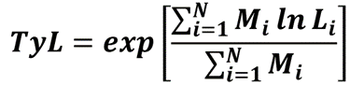
where Mi is the body mass (standardised to kilogrammes per unit area fished) of the i-th fish with length Li (in units of centimetres) in a sample of N fish.
Data for this indicator come from scientific fisheries surveys, which ideally sample the entire fish community but in practice do not. The indicator requires that surveys are conducted at regular intervals (e.g., annually) in the same area with a standard fishing gear. Sufficiency of available sample sizes can be judged using re-sampling techniques (Shephard et al., 2012, Lynam and Rossberg, 2017). The absolute biomass of individuals in length classes present in the environment is not recorded directly by surveys, rather observations are made from samples with detection error (including many false negatives). The detection error is further complicated by differing catchabilities over length classes and species such that the relative abundance between species and length classes observed is survey specific. Where available, catchability estimates can be used to attempt to correct for this component of the systematic measurement error (e.g., Fraser et al., 2007; Walker et al., 2017). However, such estimates are sparse in the scientific literature and prone to great uncertainty. Alternatively, model-based estimates of absolute species abundance can be used to rescale observed abundances for some species (entire fish communities are not usually modelled), but here model uncertainty is also great (ICES, 2014b). For simplicity, Typical Length is defined with reference to a particular sampling design with a varying limitation to the size range sampled by fishing gear. For each survey, this indicator is calculated for subdivisions that represent different habitats and communities, where possible. Although each survey may provide a slightly different perspective to the reality, the surveys themselves are standardised so that they can be assumed to provide a consistent representation of that perspective over time.
The data are collected under the national programmes and the Data Collection Framework (EC, 665/2008). Currently, the most important data sources for Typical Length are those groundfish surveys that are conducted through the International Council for the Exploration of the Sea (ICES). The International Bottom Trawl Survey (IBTS) programme in the Greater North Sea, Celtic Seas, and Bay of Biscay and Iberian Coast is particularly important since the otter trawl gear used is a general-purpose design aimed to catch both demersal and pelagic species. However, beam trawl surveys are more efficient at catching benthivorous species such as sole (Figure a) and time series of Typical Length from such surveys may be preferable should sufficient length sampling of fish be made. The two gears (otter and beam) can therefore be assumed to provide complementary perspectives of the fish community.
Data Used and Quality Assurance
The assessment draws on raw data from the ICES database of groundfish surveys (DATRAS, https://www.ices.dk/data/data-portals/Pages/DATRAS.aspx). These data have been quality controlled by OSPAR as part of this assessment process to generate a data product for assessment purposes. Time series of Typical Length for fish and elasmobranchs are derived from each available groundfish survey, where the community is separated into demersal and pelagic habitat-based feeding assemblages.
Time series of Typical Length for demersal assemblages were determined for multiple surveys carried out across four OSPAR Regions: the Greater North Sea, Celtic Seas, Bay of Biscay and Iberian Coast, and Wider Atlantic (Table a). Ecological subdivisions were determined for the Greater North Sea using a simplification of those strata proposed by the EU financed project Towards a Joint Monitoring Programme for the North Sea and Celtic Sea (JMP NS/CS) that took place in 2013, and building upon work in the EU VECTORS project (Vectors of Change in European Marine Ecosystems and their Environmental and Socio-Economic Impacts) that examined the significant changes taking place in European seas, their causes, and the impacts they will have on society. In other OSPAR Regions, the strata from the survey design were considered appropriate to represent the ecological subdivisions.
 (© Hans Hillewaert)")
Figure a: Common sole (Solea solea) (© Hans Hillewaert)
Standard data collected on these surveys consists of numbers of each species of fish sampled in each trawl haul, measured to defined length categories (i.e., so a fish with a recorded length of 14 cm would be between 14,0 cm and 14,9 cm in length). By dividing species and size-specific catch numbers-at-length by the area swept by the trawl on each sampling occasion, these catch data are converted to standardised estimates of fish density-at-length, by species, at each sampling location (i.e., trawl haul). However, the indicator is based on biomass rather than abundance, so these abundance densities have to be converted to biomass density data by applying species weight (w) at length relationships (of the form w = aLb, where a and b are species-specific parameters). Density estimates per length category per species based on biomass (kg per km2) are referred to below as catch-per-unit-area (CPUA).
These trawl-sample density-at-length estimates are averaged retaining year, species and length category information across all trawl samples within each sampling stratum (i.e., survey specific strata following the survey design, which is a rectangular grid in the Greater North Sea and generally depth-based strata elsewhere).
| Sub-region | Survey Acronym¹ | Survey Period |
|---|---|---|
| Bay of Biscay and Iberian Coast | BBIC(n)SpaOT4 | 2011 – 2018 |
| BBIC(s)SpaOT1 | 2000 – 2020 | |
| BBIC(s)SpaOT4 | 2002 – 2020 | |
| BBICPorOT4 | 2002 – 2018 | |
| BBICFraBT4 | 2011 – 2020 | |
| BBICFraOT4² | 1997 – 2020 | |
| Celtic Seas | CSFraOT4² | 1997 – 2020 |
| CSEngBT3 | 1993 – 2019 | |
| CSEngBT3 Bristol Channel | 1993 – 2020 | |
| CSIreOT4 | 2003 – 2020 | |
| CSNIrOT1 | 2008 – 2020 | |
| CSNIrOT4 | 2009 – 2020 | |
| CSScoOT1 | 1985 – 2020 | |
| CSScoOT4 | 1997 – 2020 | |
| Greater North Sea | GNSEngBT3 | 1990 – 2020 |
| GNSFraOT4 | 1988 – 2020 | |
| GNSGerBT3 | 1997– 2020 | |
| GNSBelBT4 | 2004 – 2020 | |
| GNSIntOT1 | 1983 – 2020 | |
| GNSIntOT1 Eastern Eng. Channel | 2007 – 2020 | |
| GNSIntOT3 | 1998 – 2020 | |
| GNSNetBT3 | 1999 – 2020 | |
| Wider Atlantic | WAScoOT3 | 1999 – 2020 |
| WASpaOT3 | 2006 – 2018 |
1 Survey acronym convention: first two to four capitalised letters indicate the European Union Marine Strategy Framework Directive (MSFD) sub-region (BBIC: Bay of Biscay and Iberian Coast; CS: Celtic Seas; GNS: Greater North Sea; WA: Wider Atlantic). Next capitalised and lower case letters signify the country involved (Spa: Spain; Por: Portugal; Fra: France; Eng: England; Bel: Belgium; Ire: Republic of Ireland; NIr: Northern Ireland; Sco: Scotland; Ger: Germany; Int: International; Net: The Netherlands).
International refers to the two international groundfish surveys carried out in the Greater North Sea under the auspices of ICES. In the Bay of Biscay and Iberian Coast sub-region, Spanish surveys are further delimited by (n) for surveys operating in the northern Iberian coast area and (s) for surveys operating in the southern Iberian coast area).
Next two capitalised letters indicate the type of survey (OT: otter trawl; BT: beam trawl). Final number indicates the season in which the survey is primarily undertaken (1: January to March; 3: July to September; 4: October to December).
2 This is a single survey that operates across both the Celtic Seas and the Bay of Biscay and Iberian Coast sub-regions, from the southern coast of the Republic of Ireland and down the western Atlantic coast of France. For assessment purposes this single survey was split into its two sub-regional components.
Data Treatment
Surveys with rectangular sampling grids (GNSIntOT1, GNSIntOT3, GNSNetBT3, GNSGerBT3, GNSBelBT3, GNSEngBT3, GNSFraOT4)
Catch per unit swept area (CPUA) data (kg / km2) from multiple hauls are averaged by species for each rectangular grid cell using. In the Greater North Sea these are ICES statistical rectangles, in the eastern English Channel a mini-grid (0.25° by 0.25°) is used by GNSFraOT4. The resulting rectangle-based CPUA estimates are multiplied by the area (km2) of their rectangles (using a Lambert equal area projection) to give species biomass-at-length (now measured in kg per rectangle). Subdivisional strata level (not GNSFraOT4) estimates of biomass-at-length are given by the sum of the rectangle-based biomass-at-length estimates and corrected by a scaling factor = 1 / (proportion of the area of subdivision monitored in the survey year) (units are now tonnes per subdivision). The scaling factor correction ensures that the weighting of the strata relative to each other in each year is not altered by the sampling levels. Subdivisional estimates of Typical Length are calculated at this point for investigating local responses of each assemblage.
Regional estimates of biomass-at-length are estimated from the sum of subdivisions (or in the case of GNSFraOT4 by the rectangle-based estimates). Typical Length is calculated from these data to give a survey level assessment within each region.
Surveys with Irregular Depth Banded Strata (i.e., all surveys other than those with Rectangular Sampling Grids)
Catch-per-unit-area (CPUA) data (kg/km2) from multiple hauls are averaged by species for each survey strata. Subdivisional estimates of biomass-at-length are subsequently given by CPUA multiplied by area of the survey strata (km2, using a Lambert equal area projection). Subdivisional estimates of Typical Length represent the local status of the fish community.
Regional estimates of biomass-at-length are estimated from the sum of subdivisions. The regional assessment of Typical Length is thus based on these summed subdivisional estimates.
Overall Assessment Basis
Where multiple surveys were available for assessment, key surveys were prioritised for assessment given the length of time series available and spatial coverage. If these measures were equal between surveys, then whichever surveyed the greatest biomass by assemblage was selected for indicator assessment. The following surveys were considered key:
Greater North Sea
GNSIntOT1 was selected as the key survey (preferred) for the Greater North Sea, given that it is the longest survey with the best spatial coverage. For the eastern English Channel, GNSEngBT3 was preferred given more consistent sampling here than GNSIntOT1 and GNSFraOT4.
Celtic Seas
CSScoOT1 was preferred over CSScoOT4 and CSIreOT4 due to length of time series. CSIreOT4 was preferred for subdivisions to the west of Ireland and in the northern Celtic Seas, but not in the north where there was overlap with CSScoOT1. CSFraOT4 was preferred in subdivisions of the Celtic Seas, except where overlap occurred with CSIreOT4. CSEngBT3 was preferred for the Irish Sea over CSNIrOT1 and CSNIrOT4 given the greater length of the survey.
Bay of Biscay and Iberian Coast
BBICsSpaOT1 was preferred over BBICsSpaOT4 given the length of the survey. CSBBFraOT4, BBICPorOT4 and BBICnSpaOT4 did not overlap with any other surveys. BBICFraOT4 was preferred over BBICFraBT4 due to length of survey.
Time-Series Assessment
The long-term trend in each time series (subdivision and survey level) was modelled through the application of a LOESS smoother (i.e., locally weighted scatterplot smoothing) with a simple ‘fixed span’ of one decade.
Breakpoint analyses uses data to define stable underlying periods (see Probst and Stelzenmüller, 2015). The method makes it possible to say whether there is a significant change in the time series state over time, namely whether the recent period is not significantly different from the historically observed period. The method avoids the arbitrary choice of reference periods for assessment (i.e., how many years to use to calculate an average) which can lead to subjective assessments. The shorter the period chosen, the more likely it is that noise in the data or natural fluctuations in the system are being compared against each other. However, too long a period and it could be that actual changes in state are averaged out. The minimum detectable period is defined in this analysis as six years and is assumed to be appropriate to capture the response of the fish community as opposed to noise (note that in the IA2017 assessment the minimum period was set as three years). The analysis uses two statistical approaches: First applying the ‘supremum F test’ to establish whether a non-stationary time series or a constant period for the entire time series is more suitable. If the former, then breakpoint analysis is applied to find periods of at least six years duration.
Populations should have a size structure indicative of sustainable populations and should occur at levels that ensure long-term sustainability in line with prevailing conditions. There should be no significant adverse change in the structure or function of fish assemblages due to human activities. The current assessment uses a time-series approach to identify long-term changes in state and further investigation is required to identify if reductions in the size structure of assemblages is due to human activities, food web interactions or prevailing climatic conditions. Analytical baselines are not currently available to determine assessment thresholds in terms of size-structure associated with healthy and sustainably fished assemblages. Nevertheless, fishing at Maximum Sustainable Yield in the North Sea has been shown to lead to gradual recovery in the indicator from current levels under currently prevailing conditions (Spence et al., 2021). Despite the lack of an agreed outcome for a healthy ecosystem, a lower limit can be defined based on the lowest level of the indicator observed previously. If the most recent stable period is below all previous stable states (i.e., the indicator is at the minimum observed level and the ecosystem is more dominated by small individuals than ever observed previously) the indicator cannot be said to have achieved the threshold for ‘no adverse change’. Therefore, an indicator outcome at the lowest stable state is defined as not-achieved. If the indicator has increased relative to previous periods or has not been observed to decline in the long-term the threshold ‘no adverse change’ is defined here as achieved.
Results
Greater North Sea
Mixed results in TyL were evident across the eastern English Channel. Long-term change in the longest survey (GNSEngBT3 since 1990) were evident in the UK coastal area (increase since 1997) and in the French coastal area (decrease since 2014) (Figure 2 and Figure 3). However, a strong increasing trend in the subdivision overall was apparent in GNSFraOT4 (since 1998), while the more recent GNSIntOT1 (from 2007) was variable (Figure 3 and Figure 4).
In the North Sea (including Kattegat), the longest running survey, i.e., GNSIntOT1, shows a long-term decrease to minimum levels during the 1990s prior to the start of the GNSIntOT3 survey and the beam trawl surveys (Figure 2 and Figure 4). A partial recovery from the minimum level is evident in GNSIntOT1 from the early 2000s, but this and the shorter time-series derived by GNSIntOT3 (from 1998) have been variable with no clear trend overall since then. The following overall patterns are apparent in the indicator of the North Sea: a decrease that was driven by change prior to 1990 in each subdivision (Figure 5), followed by a recovery in the two northern-most areas during the 2000s and a variable pattern with no clear trend in the 2010s.
In the more recent beam trawl data for the central and southern North Sea, a decrease overall in 2005 (Figure 4) was found in GNSNetBT3 (due to change in the central areas, Figure 6) and in the south-eastern North Sea in GNSBelBT3, Figure 7.
Celtic Seas
A mix of outcomes (increases, decreases and no change) were evident in the Celtic Seas Region (Figure 2). Overall increases were found in the Irish Sea (CSEngBT3) and Bristol Channel (CSEngBT3_Bchannel) and much of the Celtic Seas south of Ireland (CSIreOT4) (Figure 2, Figure 3 and Figure 4). However, to the south of the Region decreases were found for the deep waters at the edge of the shelf (CSFraOT4, Figure 2).
One survey, CSScoOT1, demonstrated an overall decrease in the area west of Scotland (Figure 3 and Figure 4). However, the shorter CSScoOT4 indicated signs of recovery since 2005 (Figure 3 and Figure 4). Within CSScoOT1, a small subdivision to the north of Scotland (Figure 2) was found to have increased in Typical Length during the mid-2000s as had the indicator for The Minch waters between mainland Scotland and the northern Hebrides (Figure 2). Nevertheless, the Clyde subdivision to the south-west of Scotland and the deep waters at the shelf edge remain at low values relative to the 1980s (Figure 2).
Bay of Biscay and Iberian coast
In the Bay of Biscay and Iberian Coast, five surveys showed no change overall and one, BBICSpaOT1, demonstrated an increase in southern areas of the Iberian Coast (Figure 2). Although there is no pattern overall in the Portuguese waters, there is evidence of a decrease in two southern coast subdivisions in BBICPorOT4 and an increase in one. In the northern Bay of Biscay, there is no pattern overall but two subdivisions on the shelf are increasing while TyL at the shelf edge is decreasing.

Figure 2: Spatial pattern in outcome of Typical Length indicator by subdivision for preferred surveys by Region. Purple colouring means long-term increase evident; dark blue shows decrease to minimum level; light blue shows decrease to low but not minimum level. Grey areas show areas with no long-term change evident and black area show surveys that are too short to detect long term change.
Wider Atlantic
No change overall was evident
Figure 3: Time-series of Typical Length by survey, showing LOESS smoothed patterns, where overlapping surveys within Regions are grouped.
.")
Figure 4: Time-series of Typical Length by survey showing data points, LOESS smoothed patterns and stable periods (black if constant over period assessed and red if a breakpoint is detected).
, where CW is central-west, KS is Kattegat-Skagerrak, NE is northeast, OS is Orkney-Shetland, SE is south-east and SW is south-west.")
Figure 5: Subdivisional change within the North Sea (GNSIntOT1), where CW is central-west, KS is Kattegat-Skagerrak, NE is northeast, OS is Orkney-Shetland, SE is south-east and SW is south-west.
")
Figure 6: Subdivisional change within the North Sea (GNSNetBT3)
")
Figure 7: Subdivisional change within the North Sea (GNSBelBT3)
Conclusion
There is no consistent pattern across the whole OSPAR Maritime Area.
Increases were found in the Irish Sea overall, Bristol Channel, part of Porcupine Bank, the a small subdivision to the north of Scotland and the northern Isles (Orkney and Shetland) area within the North Sea, parts of the northern Bay of Biscay and the northern Celtic Sea.
Decreases to minimum values were found in the central and southern North Sea and Kattegat and parts of the western edge of the shelf, the Clyde area and to the south of Portugal and part of the northern French coast.
Knowledge Gaps
Further work is required to evaluate appropriate baselines and assessment values for this indicator. This is necessary because any historical baseline for the fish and elasmobranch community is likely to represent an impacted state. Assessment values should preferably be identified through multi-species modelling.
Barnes et al., (2010) Global patterns in predator–prey size relationships reveal size dependency of trophic transfer efficiency Ecology, 91(1), 222–232
Boudreau P. R., L. M. Dickie (1992) Biomass Spectra of Aquatic Ecosystems in Relation to Fisheries Yield. Canadian Journal of Fisheries and Aquatic Sciences, 1992, 49:1528-1538. Available at: https://doi.org/10.1139/f92-169
Commission Regulation (EC) No 665/2008 of 14 July 2008 laying down detailed rules for the application of Council Regulation (EC) No 199/2008 concerning the establishment of a Community framework for the collection, management and use of data in the fisheries sector and support for scientific advice regarding the Common Fisheries Policy. Available at: http://data.europa.eu/eli/reg/2008/665/oj
Daufresne M., Lengfellner K. and Sommer U. (2009) Global warming benefits the small in aquatic ecosystems PNAS 106 (31) 12788-12793. Available at: https://doi.org/10.1073/pnas.0902080106
Fraser, H. M., Greenstreet, S. P. R., and Piet, G. J. 2007. Taking account of catchability in groundfish survey trawls: implications for estimating demersal fish biomass. ICES Journal of Marine Science, 64: 1800–1819
Fung, T., Farnsworth, K. D., Shephard, S., Reid, D. G., and Rossberg, A. G. 2013. Why the size structure of marine communities can require decades to recover from fishing. Marine Ecology Progress Series, 484, 155—171. Available at: https://doi.org/10.3354/meps10305
Gibert JP, DeLong JP. 2014 Temperature alters food web body-size structure. Biol. Lett. 10: 20140473. Available at: http://dx.doi.org/10.1098/rsbl.2014.0473
ICES, 2014a - Report of the Working Group on the Ecosystem Effects of Fishing Activities (WGECO). ICES Document CM 2014/ACOM:26, Copenhagen, Section 3.4.3. Available at: http://tinyurl.com/p8vwu7d
ICES. 2014b. Interim Report of the Working Group on Multispecies Assessment Methods (WGSAM), 20–24 October 2014, London, UK. ICES CM 2014/SSGSUE:11
IPCC, 2014: Climate Change 2014: Synthesis Report. Contribution of Working Groups I, II and III to the Fifth Assessment Report of the Intergovernmental Panel on Climate Change [Core Writing Team, R.K. Pachauri and L.A. Meyer (eds.)]. IPCC, Geneva, Switzerland, 151 pp.
Jennings, S., Oliveira, J. A. A. D. and Warr, K. J. (2007), Measurement of body size and abundance in tests of macroecological and food web theory. Journal of Animal Ecology, 76: 72–82. Available at: https://doi.org/10.1111/j.1365-2656.2006.01180.x
Kerr, S. R. & Dickie, L. M. 2001. The biomass spectrum: a predator– prey theory of aquatic production. New York, NY:Columbia University Press.
Lynam C.P. and A.G. Rossberg. (2017) New univariate characterization of fish community size structure improves precision beyond the Large Fish Indicator. Available at: https://doi.org/arXiv:1707.06569
Probst WN, Stelzenmüller V (2015) A benchmarking and assessment framework to operationalise ecological indicators based on time series analysis. Ecological Indicators 55: 94-106. Available at: https://doi.org/10.1016/j.ecolind.2015.02.035
Reum, J. C. P., Jennings, S. and Hunsicker, M. E. (2015), Implications of scaled δ15N fractionation for community predator–prey body mass ratio estimates in size-structured food webs. J Anim Ecol, 84: 1618–1627. Available at: https://doi.org/10.1111/1365-2656.12405
Riede, J. O., Brose, U., Ebenman, B., Jacob, U., Thompson, R., Townsend, C. R. and Jonsson, T. (2011), Stepping in Elton’s footprints: a general scaling model for body masses and trophic levels across ecosystems. Ecology Letters, 14: 169–178. Available at: https://doi.org/10.1111/j.1461-0248.2010.01568.x
Rossberg, A. G., Ishii, R., Amemiya, T. and Itoh, K. (2008). The top-down mechanism for body-mass–abundance scaling. Ecology, 89: 567–580. Available at: https://doi.org/10.1890/07-0124.1
Rossberg, A. G. (2012). A complete analytic theory for structure and dynamics of populations and communities spanning wide ranges in body size. Advances in Ecological Research, 46, 429-522
Shephard, S., Fung, T., Houle, J. E., Farnsworth, K. D., Reid, D. G., and Rossberg, A. G. 2012. Size-selective fishing drives species composition in the Celtic Sea. ICES Journal of Marine Science, 69: 223–234
Spence, M.A., Griffiths, C.A., Waggitt, J.J., Bannister, H.J., Thorpe, R.B., Rossberg, A.G. and Lynam, C.P. (2021) Sustainable fishing can lead to improvements in marine ecosystem status: an ensemble-model forecast of the North Sea ecosystem. Marine Ecology Progress Series 680:207-221. Available at: https://doi.org/10.3354/meps13870
Walker, N. D., Maxwell, D. L., Le Quesne, W. J. F., and Jennings, S. (2017) Estimating efficiency of survey and commercial trawl gears from comparisons of catch-ratios. ICES Journal of Marine Science. Available at: https://doi.org/10.1093/icesjms/fsw250
Contributors
Lead authors: Lynam, C.P., Piet, G., Volwater, J.
Supported by: Foodweb Expert Group, Intersessional Correspondence Group on the Coordination of Biodiversity Assessment and Monitoring (ICG-COBAM), and OSPAR Biodiversity Committee (BDC)
Citation
Lynam, C.P., Piet, G., Volwater, J., 2022. Size Composition in Fish Communities. In: OSPAR, 2023: The 2023 Quality Status Report for the Northeast Atlantic. OSPAR Commission, London. Available at: https://oap.ospar.org/en/ospar-assessments/quality-status-reports/qsr-2023/indicator-assessments/size-composition-fish-communities
| Assessment type | Indicator Assessment |
|---|---|
| Summary Results | https://odims.ospar.org/en/submissions/ospar_size_comp_fish_msfd_2022_06/ |
| SDG Indicator | 14.2 By 2020, sustainably manage and protect marine and coastal ecosystems to avoid significant adverse impacts, including by strengthening their resilience, and take action for their restoration in order to achieve healthy and productive oceans |
| Thematic Activity | Biological Diversity and Ecosystems |
| Relevant OSPAR Documentation | Agreement 2018-05 CEMP Guideline: FW3 Combined guideline for processing of survey data for fish and food webs common indicators FC2, FC3, FW3 and FW7 |
| Date of publication | 2022-06-30 |
| Conditions applying to access and use | https://oap.ospar.org/en/data-policy/ |
| Data Snapshot | https://odims.ospar.org/en/submissions/ospar_size_comp_fish_dsnap_2022_06/ |
| Data Results | https://odims.ospar.org/en/submissions/ospar_size_comp_fish_dres_2022_06/ |