

Changes in Plankton Diversity
Background
Marine plankton are microscopic organisms that occur mostly in the upper layers of the ocean. Monitoring plankton community composition can help improve our understanding of how sustained long-term and/or rapid changes in plankton diversity can alter marine ecosystem functioning and impact the regulating, provisioning and cultural services ecosystems provide to humans.
Phytoplankton are extremely diverse, varying from photosynthesising cyanobacteria, to plant-like green micro-algae, silicon-armoured diatoms, flagella-driven dinoflagellates, and calcite-plated coccolithophores. Like phytoplankton, zooplankton are also extremely diverse. By feeding on phytoplankton, zooplankton play a major role in the marine food web, linking phytoplankton to fish, and are thus responsible for energy transfer to higher trophic levels. Plankton species composition and abundance are continuously influenced by changes in physical, chemical, and climatic conditions. As a result, plankton community composition fluctuates in space and over very short time scales (e.g., hours/days). Climate change due to greenhouse gas emissions, pollution and/or eutrophication (i.e., excessive nutrient inputs) or removal of mid-trophic levels (by selective fishing) are mainly but not strictly human-induced disturbances. Since many species respond differently to changing environmental conditions, natural and human-induced pressures can drive changes in community composition. Consequently, the dynamics of the plankton community, and its structural attributes (e.g., diversity, dominance, size structure), will differ from those of natural (undisturbed) communities.
Due to their important and diverse roles in marine ecosystems, understanding plankton dynamics is essential for ecosystem-based management. To help assess species dominance (the most abundant taxon in relation to other taxa) which often occurs in impacted areas (e.g., Bužančić et al., 2016), an analysis of community variance is made over time and space. In closed ecosystems, sites with little change in species composition over time are characterised by minimal community variance, whereas sites which have shifted to a species-poor state, or which have experienced improvement of ecological state, are characterised by large community variance. Thus, the direction of the change in variance may be an indicator of the ecological state of pelagic communities.
To quantify changes in biodiversity, indices based on the number of species and / or their relative abundances in the community can be calculated. ‘Species richness’ was identified as an Essential Biodiversity Variable and an Essential Ocean Variable, a measurement required for studying, reporting, and managing biodiversity changes (Pereira et al., 2013). There are many indices in the scientific literature to quantify species diversity but their use in a management context depends on: the objective of the study; their ecological relevance and redundancy; the mathematical properties; and ease of interpretation by stakeholders (Rombouts et al., 2019).
Few community composition indicators of environmental status have been applied to date and this probably reflects the difficulty in setting comparison conditions and environmental objectives for these indicators (Garmendia et al., 2013). The response of phytoplankton communities to human pressures is often non-linear and not always correlative, making it difficult to identify clear state-pressure linkages. On the other hand, the main advantage of using diversity indices is their advanced development within the scientific literature and their ease of calculation.
In contrast to indicators of environmental status based on chlorophyll-a, diversity indices (based on abundance and richness) are generally calculated on the entire plankton community, including heterotrophic species, and will therefore provide additional information for assessing pelagic habitats (Domingues et al., 2008). The integration of bulk component with composition data may provide an even better understanding of environmental conditions, because the inclusion of additional metrics can increase the sensitivity of an index (Garmendia et al., 2013).
Multiple case studies have addressed the existing gaps and difficulties in applying diversity indices. Some studies have highlighted difficulties with the selection of appropriate indices (e.g., Richirt et al., 2019), while others have assessed environmental status through phytoplankton composition using multiple diversity indices (e.g., Francé et al., 2021). They recommended using three categories of indices to assess pelagic habitats: richness, evenness, and dominance. Recently, the importance of spatial and temporal scales for calculating indices has also been addressed (Francé et al., 2021, Bedford et al., 2020). As discussed in Bedford et al., (2020), the temporal scale of the assessment is very important if the assessment system requires a comparison index with regard to a comparison period. Among the plethora of other studies on diversity indices, few works were only focused on combining α- and β-diversity (e.g., Richirt et al., 2019, Mousing et al., 2016) to provide a spatio-temporal view of plankton community composition.
The current assessment of the PH3 indicator has addressed many of the knowledge gaps discussed in the previous assessment for IA 2017. This assessment has also addressed many of the suggestions and gaps highlighted by recent scientific literature in the field of diversity and conservation described in the previous paragraph. These improvements to the PH3 indicator methodology were partially developed as part of the French MSFD assessment in 2018, and are also ongoing as part of the European Union financed NEA-PANACEA project.
Plankton assemblages are generally characterised by a few common and many rare species exhibiting spatial and temporal compositional variability. Successional processes in plankton communities are driven by local to large-scale processes. Taxa undergo complex reactions and interactions response to variation in environmental conditions throughout the year, including seasonal changes in temperature, water column mixing/stratification, nutrient loading, and light availability (Chalar, 2009). Other processes undergo cycles over periods of days to weeks, such as meteorological events/conditions (wind, rain, cloudiness), and hydrological events/structures (upwelling/downwelling, hydrological withdrawal, water level fluctuations, temporary or permanent frontal structures at meso or sub-mesoscale). Over the long term, plankton assemblages also react to climate change and to large-scale processes, such as variability in atmospheric circulation patterns (e.g., North Atlantic Oscillation). Hence, it is important to consider plankton assemblages at multiple temporal and spatial scales. The study of plankton assemblages in space and time can be carried out by studying plankton diversity. This approach should however consider different elements of the community, such as biomass, species composition, taxonomic and functional diversity (Rombouts et al., 2019). Further investigations within the NEA-PANACEA project will continue the work initiated as part of the EcApRHA project to investigate the aggregation of these community elements by combining the PH1/FW5, PH2 and PH3 indicators which focus on different, but complementary, attributes of the plankton community.
Methodology and concept:
The aim of this assessment using diversity indices was not only to quantitatively describe the community composition but also to enhance the ability to detect changes in the structure of the community across seasonal and annual scales. Indices to quantify biological diversity are numerous and thus the choice of the most appropriate and the most sensitive index to calculate community diversity can be difficult. The method has been applied to deliver a common indicator assessment for the Celtic Seas. It has also been tested to produce a pilot assessment for the Greater North Sea and Bay of Biscay and Iberian Coast.
Considering several indices that focus primarily on the number of species (or richness) (e.g., Species richness (S), Menhinick (D), and Margalef (d) indices) and/or the dominance of a few species (Shannon, Berger-Parker, Patten (R), Gini (D ̂) and Hulburt (δ) indices) within the community will provide a holistic understanding of the community structure which would not be possible if these indices were to be assessed independently.
The PH3 indicator focuses on α-diversity (i.e., the diversity within a site or sample) and β-diversity, which focuses on the rate of change, or turnover, in species composition (Rombouts et al., 2019). Caution must be taken when using these as diversity indices. Firstly, indices can be biased for a number of reasons: e.g., due to sampling effort (Cozzoli et al., 2017), scale of investigation, sampling methods (Rodríguez-Ramos et al., 2014), advection of new taxa (Lévy et al., 2014), and improvements to taxonomic expertise (Dromph et al., 2013). A careful description of the level of identification and the abundance within each taxon must be given as they strongly impact the results. In addition, plankton communities do not respond linearly to anthropogenic pressures. Thus, clear state-pressure relationships are difficult to identify (Garmendia et al., 2013).
In this assessment, the Menhinick Index was chosen for assessing species richness of both phytoplankton and zooplankton communities as it is the most sensitive index to changes in environmental conditions without differentiating natural and anthropogenic sources (Budria et al., 2017, Rombouts et al., 2019). To avoid potentially biased results, species richness (S) of phytoplankton and zooplankton were not included in this assessment since they are highly correlated with sampling effort and with the level of expertise of taxonomists analysing samples.
In addition to richness, ‘dominance’ indices are also available in the literature and often highly intercorrelated. The investigations made by Budria et al., (2017) and Rombouts et al., (2019) found that the Hulburt index better describes the dominance for phytoplankton, whereas the Gini and Patten indices are more suited for zooplankton (e.g. Duflos et al., (2017). Furthermore, indices for zooplankton require further testing and validation before they can be fully accepted by the scientific community. The procedure has to identify which indices are able to identify changes in the community structure on annual and seasonal basis.
In this assessment, bimonthly plankton data from diverse sources were used (e.g., Continuous Plankton Recorder (CPR), microscopy counts, FlowCAM). Index computation was conducted separately for each dataset, and separately for zooplankton and phytoplankton. In addition, the computation of the indices was considered independently of the taxonomic level. The Menhinick, Hulburt, Gini, and Patten indices were calculated for every month. Only years with more than eight months of sample data were used. This procedure is spatially consistent with the other pelagic habitat indicators (PH1/FW5 and PH2) and with the food web indicator 2 (FW2 primary production) since the same assessment units were used. Missing data were not interpolated in this assessment, as interpolation at level of individual taxa can introduce large biases in species abundance.
The Menhinick index (D; Whittaker, 1977) measures taxonomic richness but is more sensitive to environmental change than other richness indices. The Menhinick index is given by the following equation:
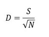
where S is the number of taxa and N is the number of individuals.
The Hulburt Index (δ; Hulburt, 1963) is a measure of dominance and is relatively easy to interpret since it is expressed as a percentage. Its formula is as follows:
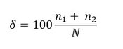
where n1 is the abundance of the dominant genus and n2 is the abundance of the second most abundant genus and N is the total abundance.
To relate the Hulburt Index to environmental pressures, the ‘100 - δ’ value was used, in line with the classic theory in which dominance phenomena and changes in community composition occur in impacted areas (Howarth et al., 2000; Facca et al., 2014).
The Gini coefficient (D ̂; Gini, 1912) is a measure of dominance. It is considered one of the best indices to describe α-diversity (Beaugrand and Edwards, 2001). The Gini coefficient is given by the formula:
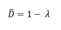
where λ is the Simpson Index, which is expressed as:
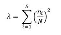
where ni is the abundance of the species i, N is the total abundance and S is the number of species in the sample.
The Patten index (R; Patten, 1962) is a measure of dominance which is sensitive to the taxonomical level of determination. Thus, the strategy of analysis should influence the calculation of this index. For the current assessment, this bias was avoided by treating each dataset separately. Each contracting parties or owner of the datasets was assumed to overcome this bias prior sending the datasets. The Patten index is described by:
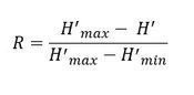
where H’ is the value of the Shannon-Weaver index for the considered sample/community, H’max is the highest value of the index among the different samples/communities and H’min is the lowest.
The Shannon-Weaver index (H’; Shannon and Weaver, 1949), which is another measure of diversity, is described by:
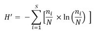
where N is the number of individuals, S is the number of species and ni is the abundance of species i.
Another category of indices exists to quantify the onset and amplitude of variation in the community structure. Temporal β-diversity is the variation in community composition with time within a study area (Legendre and Gauthier, 2014). More specifically, the Local Contribution to Beta Diversity (LCBD) indicates how much each observation in a time-series contributes to β-diversity; for example, a site with an average species composition would have an LCBD value of 0. Large LCBD values may indicate sampling units (in time) characterised by high conservation value, or degraded and species-poor sites that are in need of restoration (Legendre and De Cáceres, 2013). High values may also correspond to special ecological conditions, or may result from the disturbance effect of invasive species (i.e., differing from normal conditions in a positive or a negative way). As such, LCBD indices are comparative indicators of the ecological uniqueness of the sampling units along the time series. Temporal β-diversity was computed as the total community composition variance across years following the method described in detail by Legendre and De Cáceres (2013; Figure a).
")
Figure a: Schematic diagram representing the method used to compute β-diversity as the total variance in species composition (adapted from Legendre and De Caceres, 2013)
While the β-diversity index (LCBD) reports the temporal changes of the community and their significance, the α-diversity indices report the state of the community (Rombouts et al., 2019). Consequently, the computation of β and α-diversity are consecutive. If the β -diversity index indicates significant community change, then subsequent computation of α-diversity indices can address the nature of change to highlight whether richness, dominance, or both are responsible for the detected changes.
Detection of taxa responsible for atypical composition
When the LCBD was found significant, the detection of the taxa responsible for the atypical composition was processed using the Important Value Index (IVI). It is a measure of the importance of a taxon in terms of its relative density and frequency to the rest of the community within a given site. The IVI is computed according to the following formula:
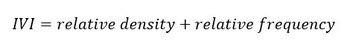
Where relative density corresponds to the abundance ratio of a given taxa over the total abundance in the sample, and relative frequency represents the proportional occurrence of the given taxa relatively to the total number of taxa considered in the sample (Curtis and McIntosh, 1950; Mukherjee et al., 2010). Its application to the PH3 indicator has been successfully demonstrated by other researchers (Duflos et al., 2018; Rombouts et al., 2019).
Integration of the α and β-diversity indices
Biological assessment results need to be expressed using a numerical between zero and one, the ‘Ecological Quality Ratio’ (EQR, van de Bund and Solimini, 2007). The computation of the EQR was done for each diversity index (phytoplankton: Menhinick, 100-Hulburt and LCBD; zooplankton: Menhinick, Gini, Patten and LCBD). The EQR makes the results for a single α and β-diversity index calculation comparable across assessment units. For each plankton component, three α and β-diversity indices were integrated and simplified into an EQR per index.
This measure compares the conditions (e.g., values of an index) of an assessment period to the conditions from a comparison period. For each previously calculated diversity index, the conditions of the comparison period (i.e., comparison values) are defined as the maximum value of each α-diversity (and 100-Hurlburt) index and the minimum value of LCBD, because these values may be associated with good ecological status of plankton communities. Values of EQR close to 0 result in conditions far from those of the comparison period, whereas values of EQR close to 1 indicate conditions close to those of the comparison period (Figure b). The EQR was applied on multiple fixed stations in the French ecological evaluation of the Pelagic Habitat in 2018 (Duflos et al., 2017). The current OSPAR PH3 assessment also employs the EQR through a continuous scale. The EQR requires further validation which will be carried out as part of the NEA-PANACEA project. We also tested the computation of a mean EQR which is the average of the EQRα and the EQRβ under a single metric. As the development of the mean EQR is still ongoing, it is only computed for fixed stations and compared to the EQRα and EQRβ.
The EQRα for dominance and richness indices is defined as:
The maximum values of dominance and richness indices are set as comparison values.
The EQRβ for LCBD is defined as:
The minimum value of LCBD is set as the comparison value since the lower the LCBD, the more evenly distributed the species.
 and its significance in relation to the comparison conditions (from Duflos et al., 2017). In the current OSPAR assessment, the EQR is used as a continuous metric, from 0 to 1 with values of EQR close to 0 indicating high dominance, low richness in the sample and “atypical” community structure. Values of EQR close to 1 indicate low dominance, high richness in the sample and “typical” community structure. Arbitrary classes were displayed as illustration.")
Figure b: Ecological Quality Ratio (EQR) and its significance in relation to the comparison conditions (from Duflos et al., 2017). In the current OSPAR assessment, the EQR is used as a continuous metric, from 0 to 1 with values of EQR close to 0 indicating high dominance, low richness in the sample and “atypical” community structure. Values of EQR close to 1 indicate low dominance, high richness in the sample and “typical” community structure. Arbitrary classes were displayed as illustration.
Kendall trend test and statistic:
The trend in annual EQRβ over time was assessed with the Kendall trend test. The test was performed on annual EQRβ values, rather than monthly or seasonal values, to account for the inter-annual variation in diversity and to remove the cyclical seasonal effects. This nonparametric test generates a statistic which is derived by comparing each value in a time-series with each of the values preceding it. If a latter value is greater than a previous one, the pairwise comparison is assigned a value of 1. If it is smaller, it is assigned a value of -1, with 0 assigned to cases when there is no difference between values. The sum of the pairwise comparisons for the time-series produces Kendall’s S-statistic. The variance in the S-statistic is used to derive a Z-score with an approximately normal distribution; thus, confidence in this statistic can be assessed with an associated p-value, with p ≤ 0,05 generally accepted as statistically significant change. The sign of the test statistic reveals the direction of the trend, with a positive or negative statistic indicating an increasing or decreasing trend, respectively. The magnitude of the statistic is proportional to the strength of the trend. A benefit of this test is that it can be applied identically to transformed and non-transformed data. It also has the advantage that trends in the EQRβ are comparable across datasets and assessment units. The Kendall trend test applied to the EQR identifies long-term / permanent (significant trend test and significant LCBD) or episodic change in composition (non-significant trend associated with significant LCBD). This test result can also be significant while the LCBD is non-significant, indicating gradual long-term or permanent changes in community composition.
Previous assessment:
For the previous assessment (OSPAR Intermediate Assessment; IA2017) a pilot assessment of the PH3 candidate indicator was produced for the Greater North Sea and the Bay of Biscay and Iberian Coast as only a small amount of data was available. The choice of the best indices to study community composition was still in an early stage of testing, especially for zooplankton where more methodological development was needed. In IA2017, the pilot assessment of PH3 was carried out using a limited amount of phytoplankton data so that the indicator could describe the state and change in phytoplankton community composition in time but not the variability in space. Building on the work carried out by Budria et al., (2016) and Duflos et al., (2017), the statistical significance of community change can now be calculated and the EQR is suggested as a measure to integrate the different diversity indices into a single value for quality status assessment. The present assessment maintains the core methodology used for IA2017 but now includes important improvements for more intuitive interpretation of the indicator results, as described above. Most of these improvements have already been tested and applied as part of the French assessment of pelagic habitat for the MSFD in 2018 (Duflos et al., 2017).
Spatial scales:
Because plankton community composition, distribution, and dynamics are closely linked to their environment, the analysis was performed at the scale of the ‘COMP4 assessment units’ (Figure c). Assessment units within the Greater North Sea and Celtic Seas (OSPAR Regions II and III, respectively) were initially developed by Deltares partner institutes as part of the EU Joint Monitoring Programme of the Eutrophication of the North Sea with Satellite data (JMP-EUNOSAT; Enserink et al., 2019) and further refined in the revision process of the eutrophication assessment by OSPAR expert groups ICG-EMO and TG-COMP. Assessment units with similar phytoplankton dynamics were derived from cluster analysis of satellite data for chlorophyll-a and primary production. Boundaries between assessment units were derived by relating clustering results to the best-matching gradients in environmental variables obtained from three-dimensional hydrodynamic Dutch Continental Shelf model version 6 (DCSMv6 FM). The variables which best matched the divisions highlighted by clustering were depth, salinity, and stratification regime. Additional geographic areas were added such as the Channel, Irish Sea and Kattegat. These assessment units are a geographical representation of the conditions which best suit plankton distribution, dynamics, and community composition.
Because the Bay of Biscay and Iberian Coast (OSPAR Region IV) extended beyond the boundaries of the DCSMv6 FM, assessment units within this Region were developed using a different methodology, based on phytoplankton dynamics (Spain) and salinity dynamics (Portugal). To delineate assessment units for the Spanish coast, a polygon was created, extending from the coast to the exclusive economic zone (EEZ) boundary. Daily MODIS-Aqua Level-2 satellite images were used to calculate climatological mean values of chlorophyll-a for each pixel. K-means clustering was then used to group pixels with similar dynamics, resulting in six distinct groupings within the main Spanish polygon. Portugal’s three Water Framework Directive assessment units were extended to the boundaries of the Portuguese EEZ. These assessment units were further divided longitudinally to separate pelagic waters from coastal waters more subject to eutrophication from river influence by applying a salinity threshold, followed by a bathymetry threshold.
Figure c: COMP4 assessment units developed by JMP-EUNOSAT and OSPAR. Available at: https://odims.ospar.org/en/submissions/ospar_comp_au_2023_01/
Classification of the pelagic habitats
Following the European Commission (2017) establishing criteria and methodological standards to determine good environmental status of marine waters, the COMP4 assessment units and the fixed-point stations are associated with particular habitat types within their corresponding OSPAR region (table a). Habitat identifications were processed following strict criteria according to surface mean salinity and their mean depth. Four habitats were identified: variable salinity habitat (corresponding to river plumes and region of freshwater influence (ROFI)), coastal habitat (nearshore areas adjacent to ROFIs with mean salinity < 34,5), shelf habitat (corresponding to offshore areas with mean depth less than 200 m and mean salinity > 34,5) and oceanic/beyond shelf habitats (corresponding to offshore areas with mean depth greater than 200 m).
| Area code | Area name | Salinity (surface mean) | Depth (mean) | Habitat type | OSPAR Region |
|---|---|---|---|---|---|
| ADPM | Adour plume | 34,4 | 87 | Variable salinity | IV |
| ELPM | Elbe plume | 30,8 | 18 | II | |
| EMPM | Ems plume | 31,4 | 19 | II | |
| GDPM | Gironde plume | 33,5 | 34 | IV | |
| HPM | Humber plume | 33,5 | 16 | II | |
| LBPM | Liverpool Bay plume | 30,6 | 15 | III | |
| LPM | Loire plume | 33,8 | 38 | IV | |
| MPM | Meuse plume | 29,3 | 16 | II | |
| RHPM | Rhine plume | 31,0 | 17 | II | |
| SCHPM1 | Scheldt plume 1 | 31,4 | 13 | II | |
| SCHPM2 | Scheldt plume 2 | 30,9 | 15 | II | |
| SHPM | Shannon plume | 34,1 | 61 | III | |
| SPM | Seine plume | 31,8 | 25 | II | |
| THPM | Thames plume | 34,4 | 22 | II | |
| CER | Coastal FR Channel | 34,2 | 33 | Coastal | II |
| CIRL | Coastal IRL 3 | 34,0 | 65 | III | |
| CNOR1 | Coastal NOR 1 | 34,3 | 190 | II | |
| CNOR2 | Coastal NOR 2 | 34,0 | 217 | II | |
| CNOR3 | Coastal NOR 3 | 32,4 | 171 | II | |
| CUK1 | Coastal UK 1 | 34,5 | 60 | III | |
| CUCK | Coastal UK Channel | 34,8 | 37 | II | |
| CWAC | Coastal Waters AC | No information | No information | IV | |
| CWBC | Coastal Waters BC | No information | No information | IV | |
| CWCC | Coastal Waters CC | No information | No information | IV | |
| ECPM1 | East Coast (permanently mixed) 1 | 34,8 | 73 | II | |
| ECPM2 | East Coast (permanently mixed) 2 | 34,5 | 43 | II | |
| GBC | German Bight Central | 33,4 | 39 | II | |
| IRS | Irish Sea | 33,7 | 65 | III | |
| KC | Kattegat Coastal | 25,7 | 21 | II | |
| KD | Kattegat Deep | 27,6 | 50 | II | |
| NAAC1A | NorAtlantic Area NOR-NorC1 | No information | No information | IV | |
| NAAC1B | NorAtlantic Area NOR-NorC1 | No information | No information | IV | |
| NAAC1C | NorAtlantic Area NOR-NorC1 | No information | No information | IV | |
| NAAC1D | NorAtlantic Area NOR-NorC1 | No information | No information | IV | |
| NAAC2 | NorAtlantic Area NOR-NorC2 | No information | No information | IV | |
| NAAC3 | NorAtlantic Area NOR-NorC3 | No information | No information | IV | |
| OC | Outer Coastal DEDK | 33,4 | 27 | II | |
| SAAC1 | SudAtlantic Area SUD-C1 | No information | No information | IV | |
| SAAC2 | SudAtlantic Area SUD-C2 | No information | No information | IV | |
| SAAP2 | SudAtlantic Area SUD-P2 | No information | No information | IV | |
| SNS | Southern North Sea | 34, 3 | 32 | II | |
| ASS | Atlantic Seasonally Stratified | 35,2 | 134 | Shelf | III, IV |
| CCTI | Channel Coastal shelf tidal influenced | 34,8 | 40 | II | |
| CWM | Channel well mixed | 35,1 | 77 | II, III | |
| CWMTI | Channel well mixed tidal influenced | 35,0 | 59 | II | |
| DB | Dogger Bank | 35,1 | 28 | II | |
| ENS | Eastern North Sea | 34,8 | 43 | II | |
| GBCW | Gulf of Biscay coastal waters | 34,6 | 53 | IV | |
| GBSW | Gulf of Biscay shelf waters | 34,9 | 107 | IV | |
| IS1 | Intermittently stratified 1 | 35,3 | 138 | II, III | |
| IS2 | Intermittently stratified 2 | 35,1 | 102 | II | |
| NAAP2 | NorAtlantic Area NOR-NorP2 | No information | No information | IV | |
| NAAPF | NorAtlantic Area NOR-Plataforma | No information | No information | IV | |
| NNS | Northen North Sea | 35,0 | 121 | II | |
| NT | Norwegian Trench | 34,1 | 349 | II | |
| SAAP1 | SudAtlantic Area SUD-P1 | No information | No information | IV | |
| SK | Skagerrak | 31,8 | 134 | II | |
| SS | Scottish Sea | 35,1 | 89 | II, III | |
| ATL | Atlantic | 35,3 | 2291 | Oceanic / Beyond shelf | II, IV, V |
| NAAO1 | NorAtlantic Area NOR-NorO1 | No information | No information | IV | |
| OWAO | Ocean Waters AO | No information | No information | IV | |
| OWBO | Ocean Waters BO | No information | No information | IV | |
| OWCO | Ocean Waters CO | No information | No information | IV | |
| SAAOC | Sudatlantic Area SUD-OCEAN | No information | No information | IV | |
| Stonehaven | No information | No information | Variable salinity | II | |
| Norderney | No information | No information | Variable salinity | II | |
| Scalloway | No information | No information | Variable salinity | II | |
| Scapa | No information | No information | Variable salinity | II | |
| Bay of Mount | No information | No information | Variable salinity | II | |
| Taw estuary | No information | No information | Variable salinity | III | |
| Bristol channel 1 & 2 | No information | No information | Variable salinity | III | |
| Milford Haven 1 & 2 | No information | No information | Variable salinity | III | |
| Carmarthen Bay 1 & 2 | No information | No information | Coastal | III | |
| Cleddau estuary | No information | No information | Variable salinity | III | |
| Cleddau river 1, 2 & 3 | No information | No information | Variable salinity | III | |
| Stour estuary | No information | No information | Variable salinity | II | |
| Carrick roads | No information | No information | Variable salinity | II | |
| Loch Ewe | No information | No information | Variable salinity | III | |
| L4 | No information | No information | Coastal | II | |
| N14 Falkenberg | No information | No information | Coastal | II | |
| Anholt | No information | No information | Coastal | II | |
| Slaggö | No information | No information | Coastal | II | |
| A17 | No information | No information | Shelf | II | |
| N14 Falkenberg | No information | No information | Coastal | II | |
| E2CO | No information | No information | Coastal | IV | |
| E3VI | No information | No information | Coastal | IV |
Plankton data
A total of 24 datasets were provided from 14 sources. Data filtering methods were applied to eliminate datasets which were out of the scope for this assessment (time-series with less than 5 years which is the minimum length necessary for accurate assessment, stations located within WFD areas or only partial plankton identification). Of the 24 datasets, 14 were retained after this pre-analysis step, 9 concerning phytoplankton abundance and 5 concerning zooplankton abundance. Data from ongoing monitoring within OSPAR assessment regions will be used in the future (e.g., VLIZ data from Belgium). To minimise bias in the calculation of these indices, each dataset was analysed separately. The datasets used for this assessment are described in Table b.
Only the datasets from PML (UK) and NLWKN (DE) were from fixed-point station times-series. The remaining datasets were station data acquired during regular monitoring transects (oceanographic cruises) from the other research institutes (e.g., SMHI, RWS, VLIZ, LLUR and IEO). Non-station data used here were acquired through the deployment of the Continuous Plankton Recorder (CPR) from the UK Marine Biological Association onboard ‘ships-of-opportunity’. In a few cases, the spatially distributed data resulted in localised groupings of samples being extrapolated across much larger assessment units (see distribution of CPR samples in Figure d in the PH1 indicator assessment ), as was the case for CPR data along the west of Scotland (Intermittently Stratified 1) and Ireland (Atlantic Seasonally Stratified).
| Contracting Party | Institute | Dataset name | Date range |
|---|---|---|---|
| Germany | Bundesamt für Seeschifffahrt und Hydrographie (BSH) | BSH_Phyto_Zoo | 2008-2011 |
| Landesamt für Landwirtschaft, Umwelt und ländliche Räume des Landes Schleswig-Holstein (LLUR) | OSPAR_LLUR-SH_2010-2020 | 2010-2020 | |
| Niedersächsischer Landesbetrieb für Wasserwirtschaft, Küsten und Naturschutz (NLWKN) | OSPAR_NLWKN_1999-19_phyto | 1999-2019 | |
| Spain | Instituto Espanol de Oceanografia (IEO) | IEO_RADIALES_Phyto | 1989-2016 |
| IEO_RADIALES_Zoo | 1991-2018 | ||
| Sweden | Swedish Meteorological and Hydrological Institute (SMHI) | National data_SMHI_Kattegat-Dnr: S/Gbg-2021_116_phyto | 1989-2021 |
| National data_SMHI_Kattegat-Dnr: S/Gbg-2021_116_zoo | 1996-2020 | ||
| National data_SMHI_Skagerrak-Dnr: S/Gbg-2021_116_phyto | 1986-2020 | ||
| National data_SMHI_Skagerrak-Dnr: S/Gbg-2021_116_zoo | 1996-2020 | ||
| United Kingdom | Centre for Environment, Fisheries and Aquaculture Science (Cefas) | Cefas SmartBuoy Marine Observational Network - UK Waters Phytoplankton Data 2001-2019 | 2001-2019 |
| Environment Agency (EA) | EA PHYTO 2000-2020 | 2000-2020 | |
| Marine Biological Association (MBA) | CPR dataset 1960-2019 | 1960-2019 | |
| Marine Scotland Science (MSS) | MSS Scalloway Phytoplankton dataset | 2000-2018 | |
| MSS Loch Ewe Phytoplankton | 2000-2020 | ||
| MSS Loch Ewe zooplankton | 2002-2017 | ||
| MSS Scapa Phytoplankton dataset | 2000-2020 | ||
| MSS Stonehaven Phytoplankton | 2000-2020 | ||
| MSS Stonehaven zooplankton | 1999-2020 | ||
| Plymouth Marine Laboratory (PML) | PML_L4 phytoplankton | 1992-2020 | |
| PML_L4 zooplankton | 1988-2020 | ||
| Scottish Association for Marine Science (SAMS) | SAMS-LPO-Phyto-Dec2021 | 1970-1981 | |
| 2000-2017 |
Relationship between environmental pressures and plankton diversity
Environmental variables were selected according to their relevance to determine the most important pressure in plankton diversity. The set of environmental variables used originated from different models targeting the North-East Atlantic area (Table c). The link between the PH3 and the pressures was done using the LCBD results as previous studies have demonstrated the ability to link environmental parameters to the LCBD (Vilmi et al., 2017). The EQRβ was used to maintain consistency and harmonisation among the COMP4 units.
The first step consisted in evaluating long-term links to pressures and to avoid excluding the first several decades of many plankton time-series due to missing values. To achieve this, the method used multiple random forest regressions to impute missing values based on collinearities among observed values in the predictors. For each variable containing missing values the algorithm generated a separate regression model based on all the other predictors. To improve imputation performance, a numeric variable representing ‘month’ was included in this step to better predict the consistent seasonal patterns in some variables. This step was performed using ‘missRanger’ R package (Mayer and Mayer 2019).
Then, values for each environmental variable were calculated as the mean of monthly mean gridded values (modelled and remotely sensed) within each COMP4 assessment unit. For fixed-point stations, mean values were calculated from all measurements within a 5-nautical mile radius of the station. Where in-situ data were available (total nitrogen, nitrate, phosphate, total phosphorous, silicate) they were evaluated instead of the modelled environmental variables. For Atlantic Multidecadal Oscillation (AMO) and monthly North Atlantic Oscillation (NAO), monthly values were applied identically across all assessment units since these variables have basin-scale influence likely to cover the entire assessment region.
Finally, the random forest algorithm was applied to determine the best combination of environmental variables for predicting plankton diversity without collinearity test performed prior to analysis. The algorithm is based on the combination of predictions made by multiple regression trees (in this case, k = 1000 trees) with the optimal tree (defined as the best combination of variables) obtained by majority voting.
Prior to analysis, the original datasets were split in two subsets resulting in a training set and a test set. The training set was used for the selection of the best combination while the test set was used to validate the predictions. The training set consisted of data from the comparison period (prior to 2015) while the test set consisted of data from the assessment period (from 2015 to 2019).
For map visualisation, some variables were aggregated together. Total nitrogen, nitrate, phosphate, total phosphorus, N:P ratio and silicates were pooled under the term "nutrient”. The same procedure was applied for AMO and NAO which were pooled under the term "Climate indices".
Table c: List of environmental variables used as pressures.
| Variable name | Description | Abbreviation | Source |
| Sea surface temperature | Temperature of surface layer, as measured by satellite | sst | International Comprehensive Ocean-Atmosphere Data Set (ICOADS): https://psl.noaa.gov/data/gridded/data.coads.1deg.html |
| Salinty | Salinity of the surface area | sal | European Regional Seas Ecosystem Model (ERSEM; NWSHELF_MULTIYEAR_PHY_004_009; https://doi.org/10.48670/moi-00059) |
| Total oxidised nitrogen | Total oxidised nitrogen concentration in surface layer | totn | In situ data from Marine Scotland Science (MSS): https://doi.org/10.7489/1881-1 |
| Nitrate | Nitrate concentration of the surface layer | ntra | European Regional Seas Ecosystem Model (ERSEM; NWSHELF_MULTIYEAR_BGC_004_011): https://doi.org/10.48670/moi-00058); In situ data from Plymouth Marine Laboratory (PML): https://www.westernchannelobservatory.org.uk/l4_nutrients.php |
| Phosphate | Dissolved inorganic phosphate concentration of the surface layer | phos | European Regional Seas Ecosystem Model (ERSEM; NWSHELF_MULTIYEAR_BGC_004_011): https://doi.org/10.48670/moi-00058); In situ data from Plymouth Marine Laboratory (PML): https://www.westernchannelobservatory.org.uk/l4_nutrients.php |
| Total phosphorous | Total dissolved inorganic phosphorous concentration of the surface layer | totp | In situ data from Aarhus University (Svendsen et al., 2005) |
| N:P ratio | The ration of molar nitrogen concentration to molar phosphorus concentration | np | Derived from: European Regional Seas Ecosystem Model (ERSEM; NWSHELF_MULTIYEAR_BGC_004_011): https://doi.org/10.48670/moi-00058); In situ data from Plymouth Marine Laboratory (PML): https://www.westernchannelobservatory.org.uk/l4_nutrients.php and Marine Scotland Science (MSS): https://doi.org/10.7489/1881-1 |
| Silicate | Dissolved silicates concentration of the surface layer | Si | In situ data from Marine Scotland Science (MSS): https://doi.org/10.7489/1881-1; |
| Wind speed | Wind speed (proxy of turbulence) | wspd | International Comprehensive Ocean-Atmosphere Data Set (ICOADS); https://psl.noaa.gov/data/gridded/data.coads.1deg.html |
| Mixed layer depth | Surface layer in which density is nearly homogenous wth depth | mld | European Regional Seas Ecosystem Model (ERSEM; NWSHELF_MULTIYEAR_PHY_004_009; https://doi.org/10.48670/moi-00059) |
| Light attenuation | The extinction coefficient for the vistibile light in the water column | attn | European Regional Seas Ecosystem Model (ERSEM; NWSHELF_MULTIYEAR_BGC_004_011): https://doi.org/10.48670/moi-00058) |
| Precipitation | Rate of precipitation | precip | International Comprehensive Ocean-Atmosphere Data Set (ICOADS); https://psl.noaa.gov/data/gridded/data.coads.1deg.html |
| Current velocity | Current velocity in the surface layer | cvel | European Regional Seas Ecosystem Model (ERSEM; NWSHELF_MULTIYEAR_PHY_004_009; https://doi.org/10.48670/moi-00059) |
| pH | Sea water pH reported on total scale | pH | European Regional Seas Ecosystem Model (ERSEM; NWSHELF_MULTIYEAR_BGC_004_011): https://doi.org/10.48670/moi-00058) |
| Monthly NAO | The North Atlantic Oscillation is a weather phenomoenon over the North Atlantic Ocean of fluctuations in the difference of atmospheric pressure at sea level between the Icelandic Low and the Azores High | nao | National Oceanic and Atmospheric Administration (NOAA): https://www.ncdc.noaa.gov/teleconnections/nao/ |
| AMO | The Atlantic Multidecadal Oscillation is the theorised variability of the sea surface temperature of the North Atlantic Ocean on the timescale of several decades | amo | National Oceanic and Atmospheric Administration (NOAA); https://psl.noaa.gov/data/timeseries/AMO/ |
Addressing PH3 quality status
To deliver a clear and comprehensive message to the scientific and non-scientific community, the results of the indicator were summarised by their quality status. The quality status had been defined by the change in indicator value according to assessment threshold and / or the impact of anthropogenic pressures and climate change on the indicator change (McQuatters-Gollop et al., 2022). Thus, the quality status resulted in 4 categories: Not good, Unknown, Good and Not assessed. Table d provides a detailed explanation of the different categories.
| Quality Status Categories | |
|---|---|
| Not good | Indicator value is below assessment threshold, or change in indicator represents a declining state, or indicator change is linked to increasing impact of anthropogenic pressures (including climate change), or indicator shows no change but state is considered unsatisfactory |
| Unknown | No assessment threshold and/or unclear if change represents declining or improving state, or indicator shows no change but uncertain if state represented is satisfactory |
| Good | Indicator value is above assessment threshold, or indicator represents improving state, or indicator shows no change but state is satisfactory |
| Not assessed | Indicator was not assessed in a region due to lack of data, lack of expert resource, or lack of policy support |
Results
Changes in diversity were addressed at the regional scale by assessing long-term changes in CPR data (1960-2019) and at local scale from fixed monitoring stations (1989-2019). To compare community composition across the assessment units, β-diversity was integrated through a yearly Ecological Quality Ratio (EQRβ). Whilst in assessment the PH3 has been adopted as a common indicator in the Celtic Seas, the PH3 remained a pilot assessment in the Greater North Sea and the Bay of Biscay and Iberian Coast. However, results obtained in the different OSPAR Regions are showed here.
From 2015 to 2019 on an annual basis for the 64 COMP4 assessment units and 20 stations (from fixed-stations and stations from regular monitoring campaigns), a total of 189 calculations were undertaken across phytoplankton datasets (Figure 1; 2015: 41; 2016: 42; 2017: 39; 2018: 36 and 2019: 31). 70% of the EQRβ were low (n = 132) indicating an atypical composition compared to the comparison period (before 2015). 23% of the EQRβ were intermediate indicating that the composition of the assessment period was moderately different to the composition of the comparison period. Finally, in 10 out of 189 assessment sites (COMP4 and stations), the EQRβ was higher than 0,6 revealing that the composition was very close to the comparison period. Despite the large numbers of low EQR values, only one area had significant atypical composition (CWMTI; LCBD p-value < 0,05; Figure 1). The Kendall trend test informed that only IRS (Irish Sea; the Celtic Seas) displayed a decreasing trend in EQR (Z-score = -1; p-value < 0,05) suggesting a soft but long-term change in composition. The non-significant Kendall trend test result for CWMTI unit indicated that the composition change was episodic.
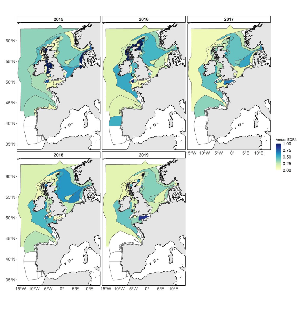
Figure 1: Evolution of the annual EQRβ of phytoplankton indices during the assessment period (2015–2019). Low EQRβ indicating large difference between the comparison value of EQRβ and the annual EQRβ value are displayed in yellow; High EQRβ indicating slightly difference between the comparison value of EQRβ and the annual EQRβ value are displayed in dark blue. White areas indicate no data or insufficient data to assess the area. COMP4 units with significant atypical composition (LCBD p-value < 0,05) are displayed as dashed areas. Monitoring fixed stations with significant atypical composition (LCBD p-value < 0,05) are displayed as dark dots. Results of Intermittently Stratified 1 (Scotland) and Atlantic Seasonally Stratified (Ireland) assessment units should be interpreted cautiously as CPR samples were extrapolated across much larger assessment units. This is a hybrid figure showing results of the common indicator assessment for the Celtic Seas and for the pilot assessment for the Greater North Sea and the Bay of Biscay and Iberian Coast.
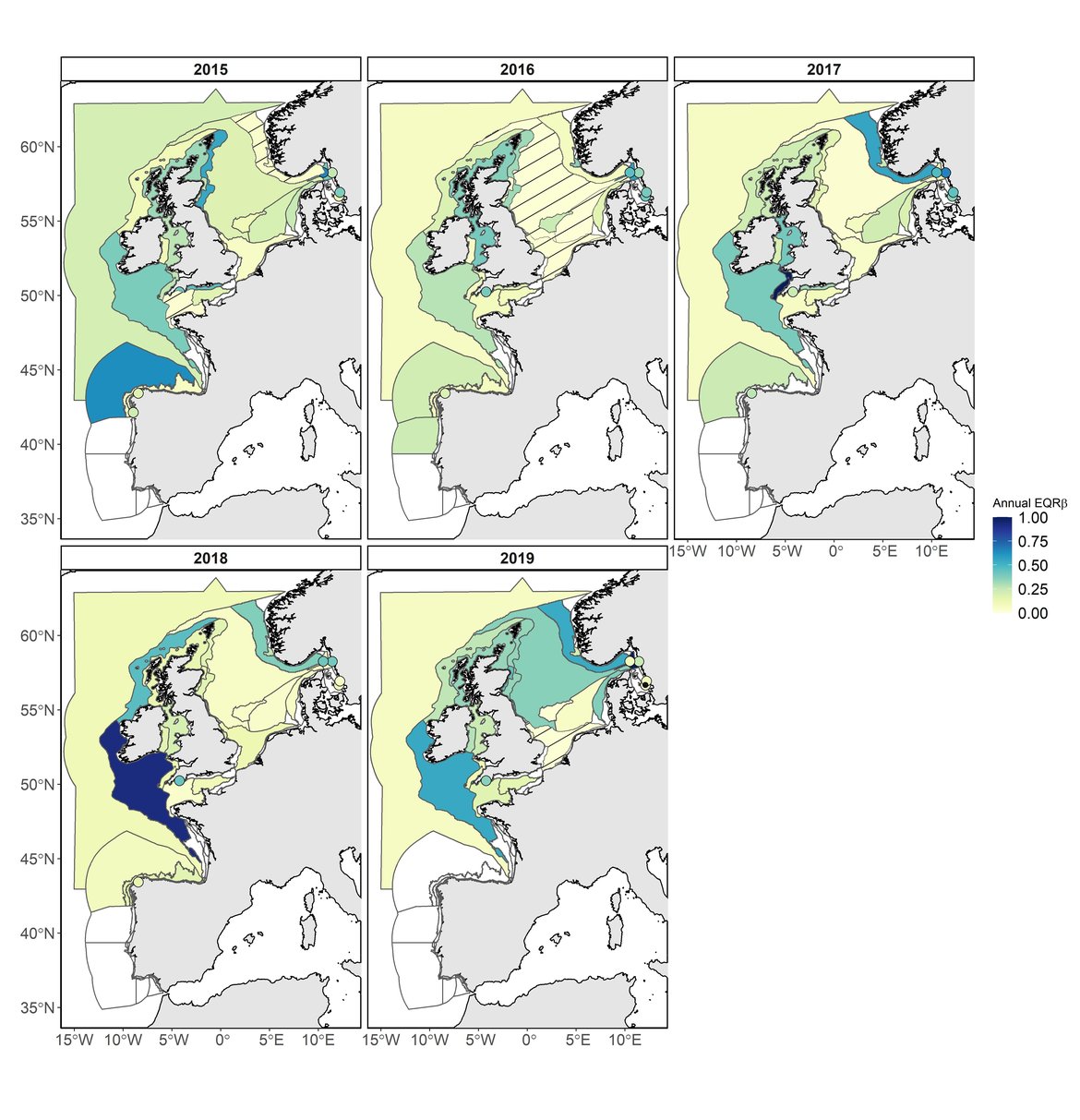
Figure 2: Evolution of the annual EQRβ of zooplankton during the assessment period (2015–2019). Low EQRβ indicating large difference between the comparison value of EQRβ and the annual EQRβ value are displayed in yellow; High EQRβ indicating slightly difference between the comparison value of EQRβ and the annual EQRβ value are displayed in dark blue. White areas indicate no data or insufficient data to assess the area. COMP4 units with significant atypical composition (LCBD p-value < 0,05) are displayed as dashed areas. Monitoring fixed stations with significant atypical composition (LCBD p-value < 0,05) are displayed as dark dots. Results of Intermittently Stratified 1 (Scotland) and Atlantic Seasonally Stratified (Ireland) assessment units should be interpreted cautiously as CPR samples were extrapolated across much larger assessment units. This is a hybrid figure showing results of the common indicator assessment for the Celtic Seas and for the pilot assessment for the Greater North Sea and the Bay of Biscay and Iberian Coast.
For zooplankton, a total of 147 calculations were undertaken (64 COMP4 units and 20 stations; Figure 2; 2015: 32; 2016: 32; 2017: 29; 2018: 29 and 2019: 25). 4% of the EQRβ (n = 6) were high, indicating that composition was close to the comparison period. 13% of the EQRβ (n = 19) were intermediate indicating that the composition of these sites (COMP4 and stations) was moderately different to one of the comparison periods. Finally, in 122 out of 147 of the assessment sites (83%), the EQRβ was low, revealing very different composition relative to the comparison period. Among the 12 lowest EQRβ values, 8 sites (CWM: 2015; NT: 2015; ECPM1: 2016; ENS: 2016; NNS: 2016; SNS: 2016; SNS and Anholt station in 2019) mostly in the Greater North Sea, had significant LCBD (p-value < 0.05; Figure 2) revealing an atypical composition. Trends were non-significant suggesting that changes in composition remained episodic.
Links between phytoplankton (Figure 3) and zooplankton (Figure 4) diversity and pressures provided evidence for the impact of climate variables. Natural climate variability (e.g., AMO) was a strong link for both phytoplankton and zooplankton in the Bay of Biscay and Iberian Coast. Decrease in pH was also highly positively correlated with the phytoplankton diversity in coastal habitats of the Celtic Seas. Nutrients (a proxy for eutrophication and water quality) were also linked directly and indirectly to the phytoplankton communities in variable salinity habitat of the Greater North Sea, coastal habitats of the Celtic Seas and shelf habitats of the Celtic Seas and the Bay of Biscay and Iberian Coast. These relationships indicate that the quality status of variable salinity habitat of the Celtic Seas was "Not good" in contrast to the “Unknown” quality status of shelf habitats of the Celtic Seas. Further details of these results can be found in the extended results, since this integration approach may obscure local relationships.
Figure 3: Most important variables addressing changes in phytoplankton diversity during the assessment period (2015-2019) within the COMP4 assessment units. This is a hybrid figure showing results of the common indicator assessment for the Celtic Seas and for the pilot assessment for the Greater North Sea and the Bay of Biscay and Iberian Coast. Available at: https://odims.ospar.org/en/submissions/ospar_changes_plank_div_var_2023_06_001/
Figure 4: Most important variables addressing changes in zooplankton diversity during the assessment period (2015-2019) within the COMP4 assessment units. This is a hybrid figure showing results of the common indicator assessment for the Celtic Seas and for the pilot assessment for the Greater North Sea and the Bay of Biscay and Iberian Coast. Available at: https://odims.ospar.org/en/submissions/ospar_changes_plank_div_var_2023_07_001/
In the previous assessment (OSPAR Intermediate Assessment; IA2017), diversity indices were computed on a monthly and annual basis to report seasonal and inter-annual changes, respectively. This descriptive methodology was inadequate for assessing spatial comparisons among assessment units. Recent improvement through the use of the EQR for the French MSFD was applied by Duflos et al., (2017). The use of the EQR makes it possible to integrate the information of diversity indices and compare the quality status across the assessment units directly. Further developments are required, by integrating the direct effect of sampling effort, while correcting indices with the Hill approach.
Investigation of nature of change: relation between α- and β-diversity and computation of the IVI
Phytoplankton diversity
Significant result coincided with the lowest EQRβ value obtained as well as low α-diversity (D = 0,01 and 100-δ = 19). However, this significant result is due to the large variation of the number of months assessed between years.
Zooplankton diversity
Across the OSPAR regions, the pilot assessment of the Greater North Sea was the only case where significant change in the indicator was detected. Winter months were generally characterised by the highest richness compared to other seasons. A strong seasonal pattern was observed for each area. Richness was higher in winter in the CWM (Figure d), NNS (Figure f), ENS (Figure g), ECPM1 (Figure e) and SNS units (Figure h) than during spring or summer. The strongest seasonal pattern was observed in the CWM, NNS and ENS units, while for the ECPM1 and SNS units it was less variable. While ECPM1 and NNS had the same richness pattern since 1960, periods of change were observed for the other spatial units. In the CWM unit, a first change occurred in the 80’s with increasing richness in early winter months while a second change occurred in 2007 with increasing richness in late winter months. These changes were not due to changes in sampling efforts as the number of samples remained equal between years. In the SNS unit, a first change happened in the 90’s with increasing richness in early winter months, while a second change was detected around 2010 with increasing richness in late winter months. Finally, in the ENS unit, richness increases occurred for early winter months around 2000 and for late winter months around 2007.
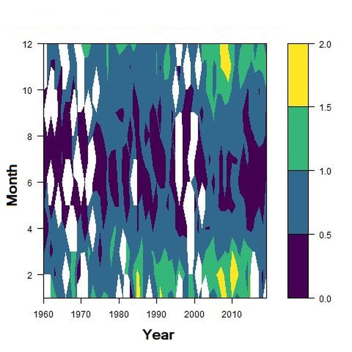
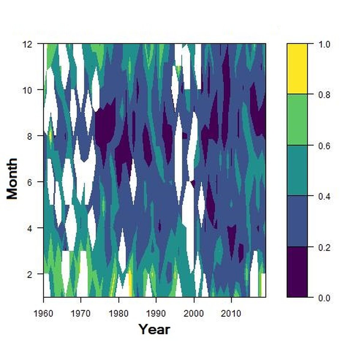
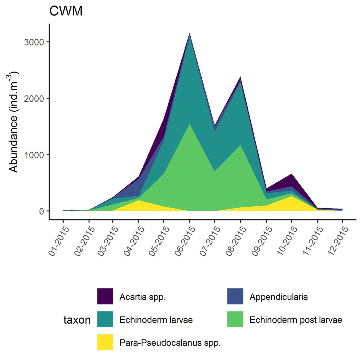
Figure d: Interannual Menhinick Richness index (left) and Patten dominance index (middle) per month and Important Value Index in 2015 (IVI; right) within the CWM unit.
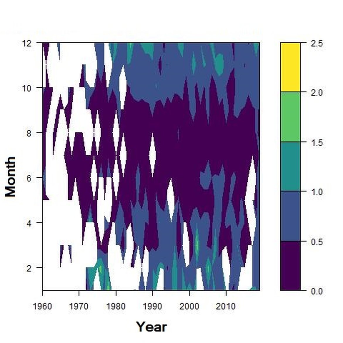
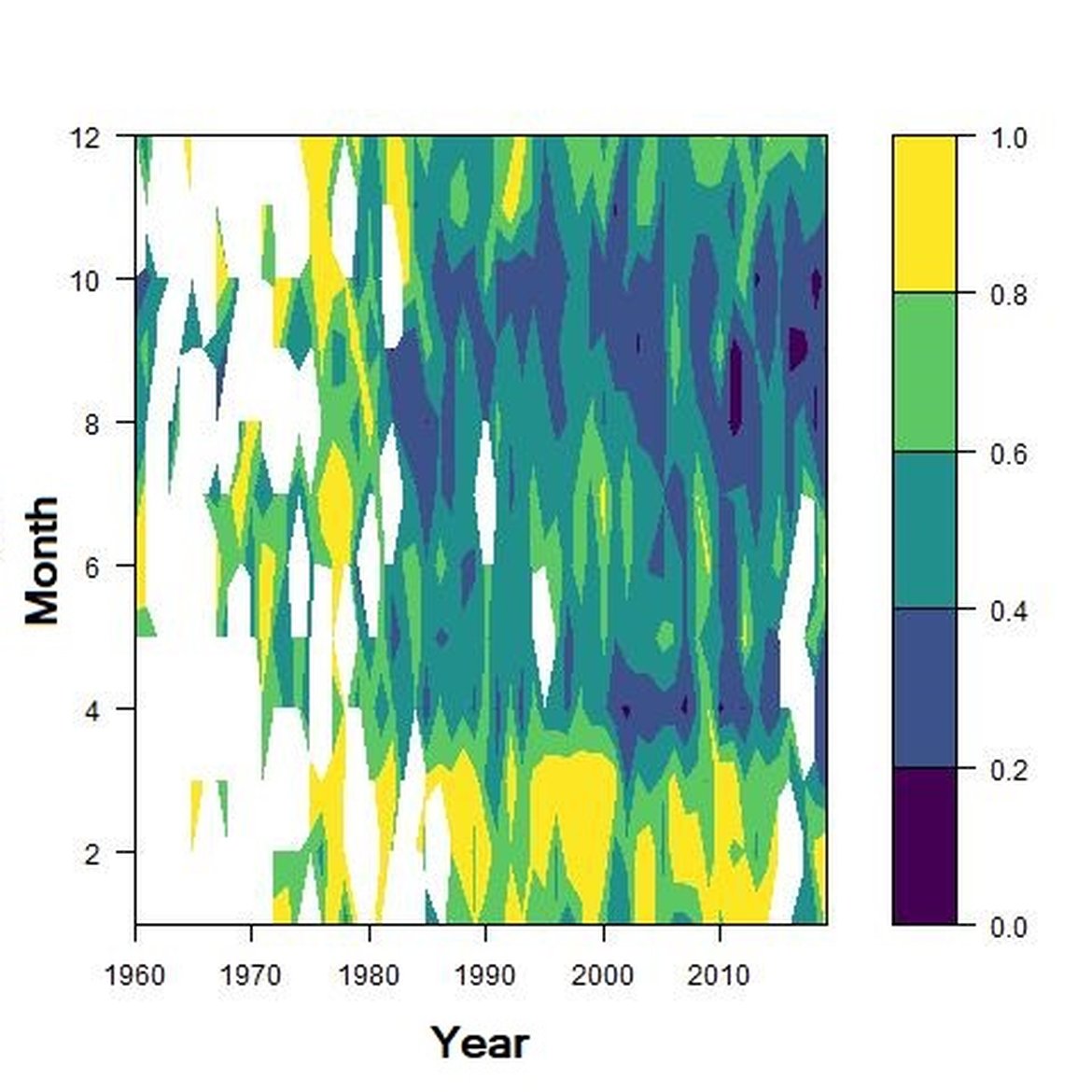
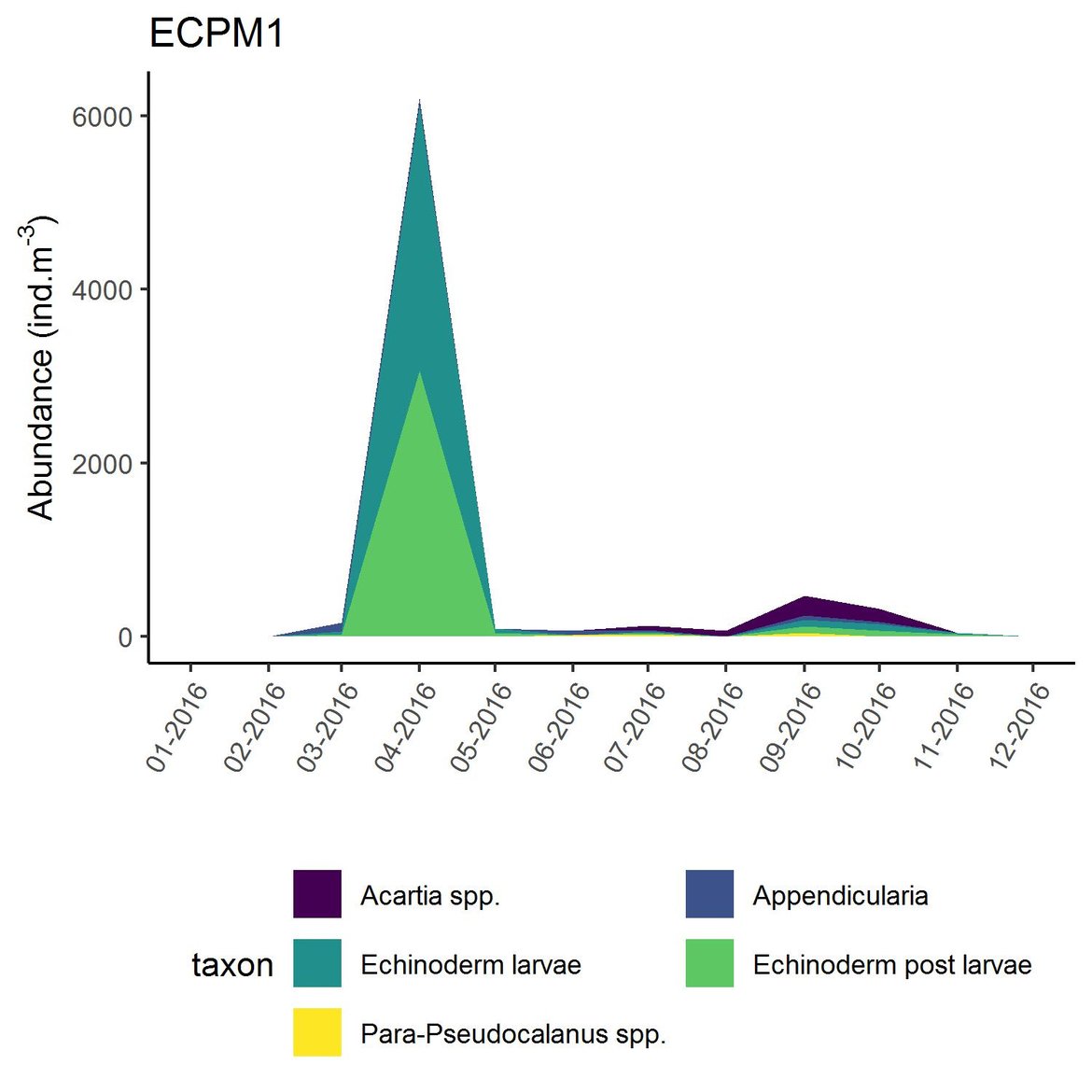
Figure e: Interannual Menhinick Richness index (left) and Patten dominance index (middle) per month and Important Value Index in 2016 (IVI; right) within the ECPM1 unit.
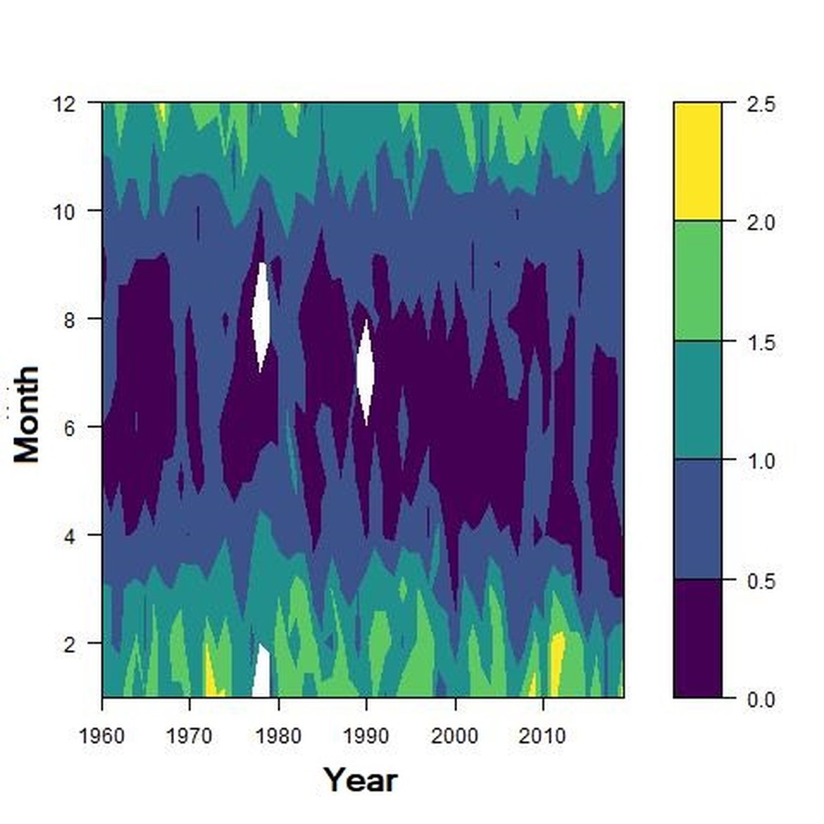
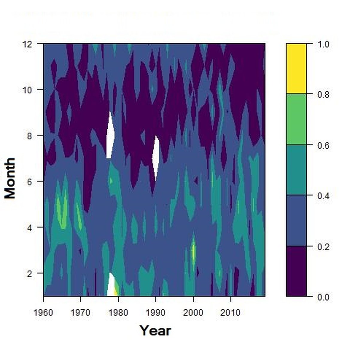
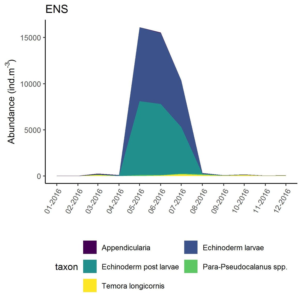
Figure f: Interannual Menhinick Richness index (left) and Patten dominance index (middle) per month and Important Value Index in 2016 (IVI; right) within the NNS unit.
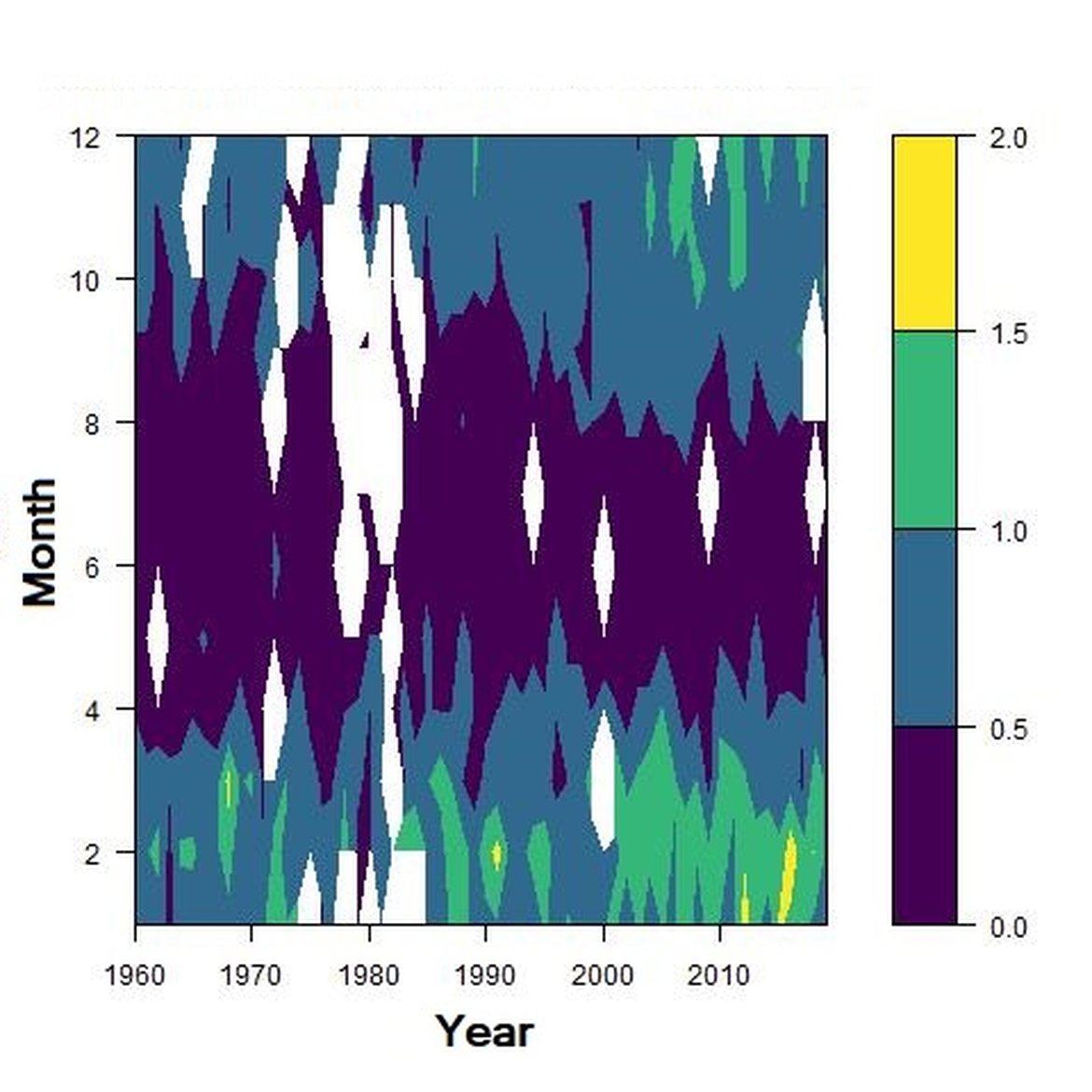
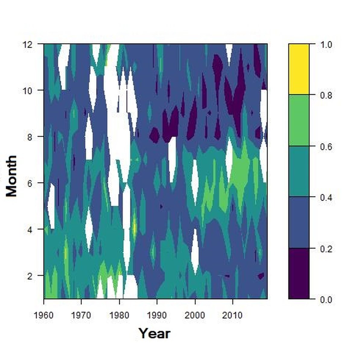
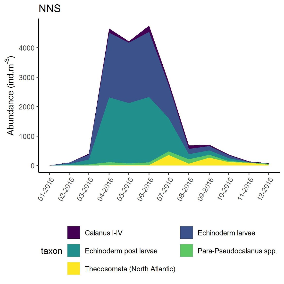
Figure g: Interannual Menhinick Richness index (left) and Patten dominance index (middle) per month and Important Value Index in 2016 (IVI; right) within the ENS unit.
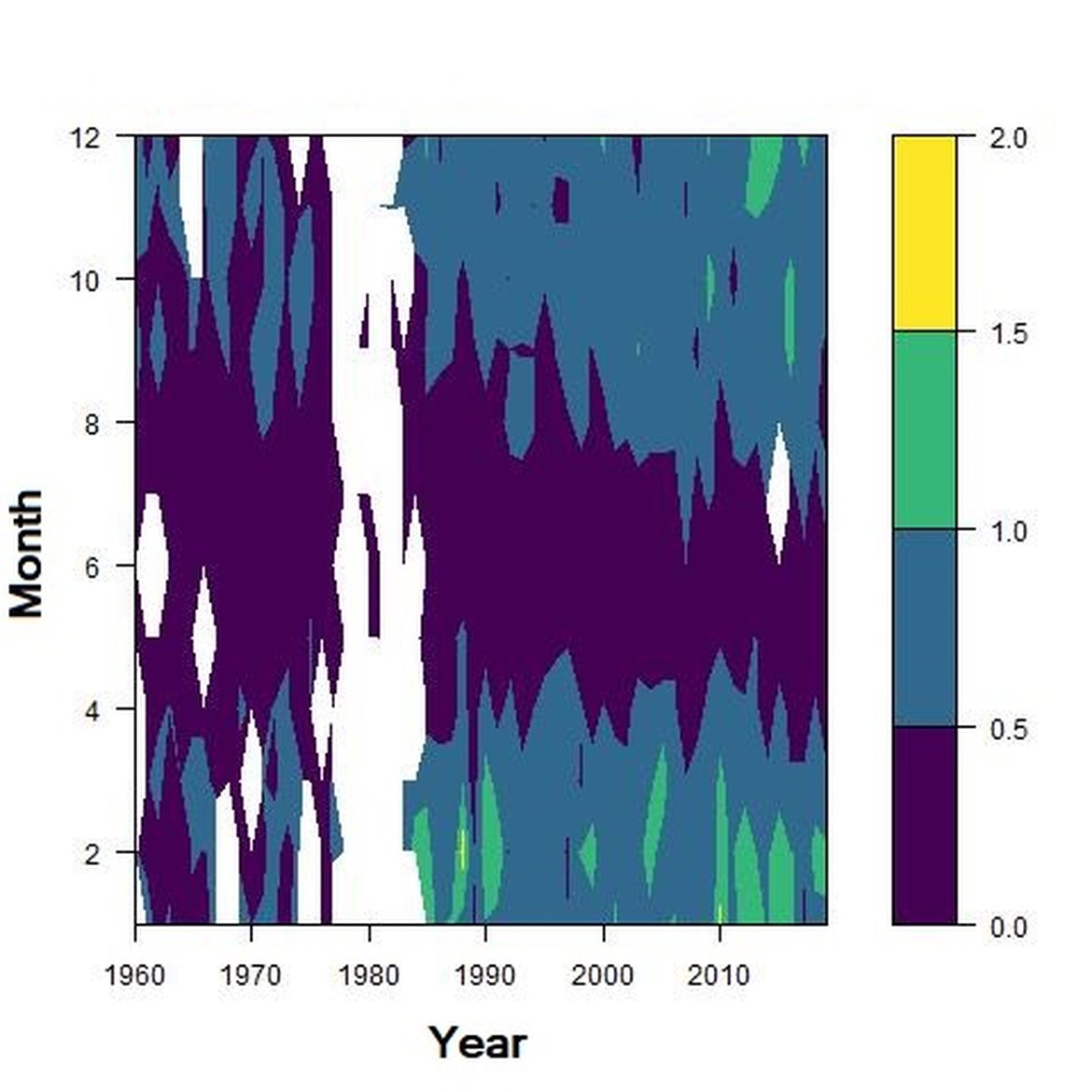
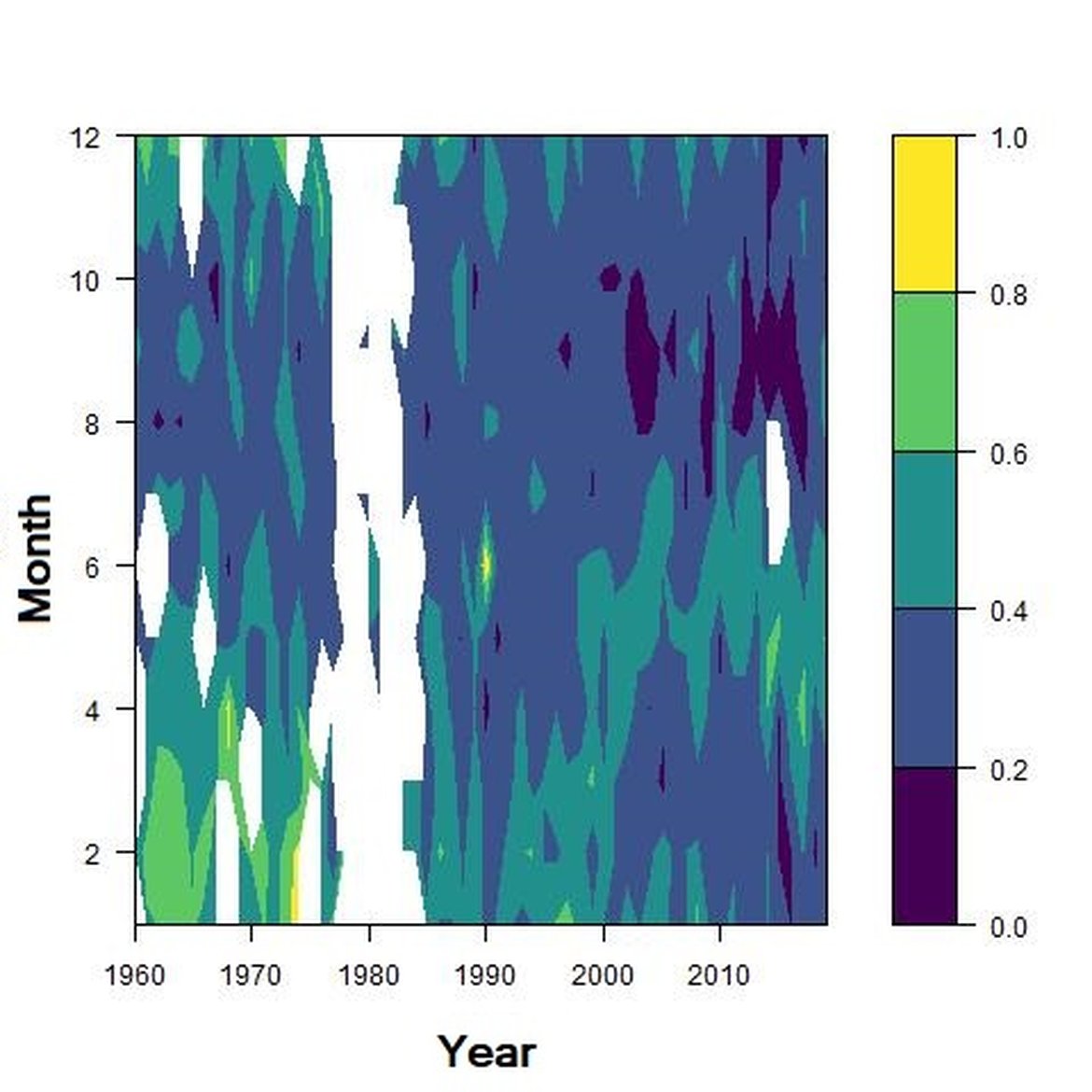
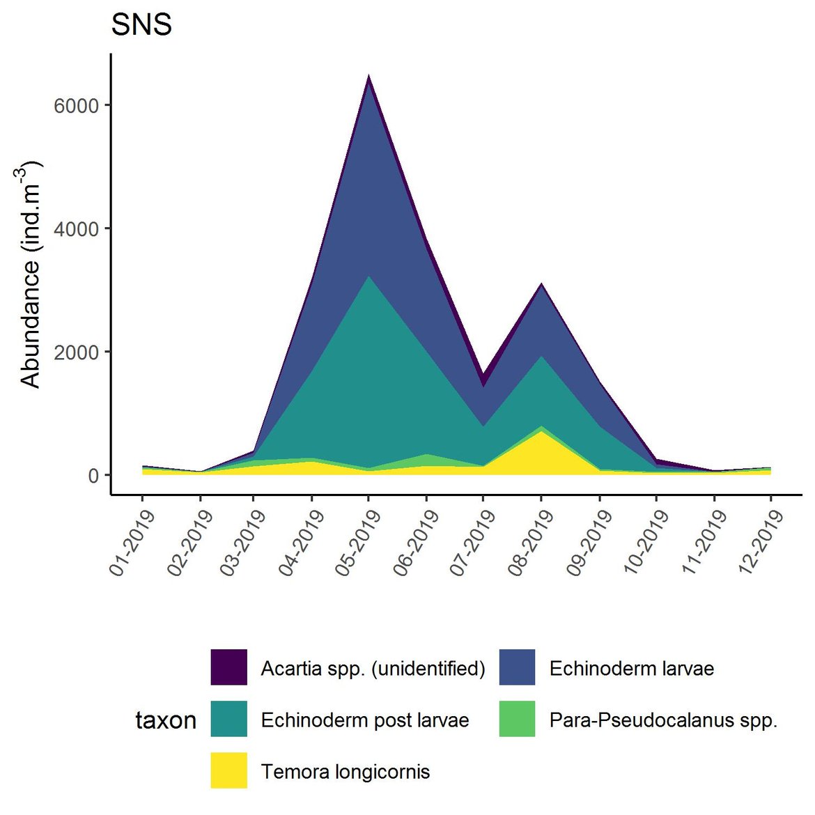
Figure h: Interannual Menhinick Richness index (left) and Patten dominance index (middle) per month and Important Value Index in 2019 (IVI; right) within the SNS unit.
Regarding the dominance, the patterns were less clear. It was apparently higher for winter months in the CWM, ECPM1 and SNS units. Some shifts in dominance within years were evident. For example, in the CWM, ENS and SNS units, the dominance shifted from winter to summer around the year 2000. In ECPM1, dominance was high in winter and summer until 1985. After 1985, summer dominance began to decrease. In the NNS, dominance was high in spring and remained consistent since 1960.
Within the different spatial units presented above, the assessment period exhibited atypical years. The IVI detected the five most important taxa responsible of the atypical composition. It is important to note that the highest IVI also corresponds to the highest dominance. The most important taxa were Acartia spp. (ECPM1, CWM, SNS), appendicularians and echinoderms larvae (ENS), and Calanus spp. (NNS). Further analyses should determine the factors responsible for this shift and the ecological relevance of these taxa in ecosystem functioning.
Computation on fixed-points stations and relation between the EQRα, EQRβ and mean EQR
In addition to spatio-temporal analysis (i.e., CPR dataset), in the pilot assessment of the Greater North Sea, examples of the EQR computed for each index at different fixed-point stations were displayed for phytoplankton (Figure i) and zooplankton (Figure j). For phytoplankton, the average EQR of station ‘Norderney’ (located in the German North Sea) was always higher than average EQR of ‘L4’ (located in the Channel Well Mixed unit). Both stations exhibited similar diversity dynamics over time. Menhinick EQR tended to increase, whereas 100-Hulburt EQR showed a decrease trend at both stations. This indicates unexpected increases in richness and dominance. Further investigation of the number of species (S) must be carried out as it may explain the increasing Menhinick EQR. The LCBD EQR was high in 2011 and 2012, revealing that the sites had a ‘common community composition’ before decreasing since 2012 towards an ‘uncommon community composition’ (e.g., Dansereau et al., 2021). Put in simpler terms, the higher the EQR of the LCBD is, the lower the LCBD, and thus the lower the rate of change in species composition. Consequently, the mean of EQRs showed that the conditions were intermediate but the EQR and consequently, the diversity, tended to decrease, congruent with the 100-Hulburt EQR.
.")
Figure i: Evolution of Menhinick EQR, Hulburt EQR, the LCBD EQR and the mean EQR for phytoplankton samples at station L4 and NLKWN. Horizontal dotted lines represent the average EQR index of the whole time series. The vertical dotted line represents the start of the assessment period (2015).
For zooplankton, patterns observed in the EQR for non-station data (i.e., the CPR; Figure 2) were also observed for fixed-point station datasets (Figure j). The richness quantified at Släggö (Kattegat) was lower than richness at L4 (Western English Channel) and RAD_3 (Iberian coast). Variations in zooplankton were more complex to interpret than for phytoplankton. A combination of effects may be responsible for such complex patterns (e.g., predator-prey interactions and fluctuations in environmental parameters, especially in coastal areas). Further investigation is required to draw connections with the pressures responsible for driving these changes, however this will be resource dependent. Connection with other relevant pelagic and food web indicators should help to address changes in zooplankton community composition.
. Horizontal dotted lines represent the average index EQR for the whole time-series. The vertical dotted line represents the start of the assessment period (2015).")
Figure j: Evolution of Menhinick EQR, Patten EQR, LCBD EQR and mean EQR for zooplankton samples at station L4, Släggö and a Rad_3 (a station from the Iberian coast). Horizontal dotted lines represent the average index EQR for the whole time-series. The vertical dotted line represents the start of the assessment period (2015).
Linking pressures and the PH3
Previous studies have demonstrated the ability to link environmental parameters to the LCBD (Vilmi et al., 2017). Therefore, it is also possible to link the environmental parameters to the LCBD EQR because the EQR is simply a harmonisation of the LCBD allowing for the comparison between the COMP4 assessment units. As a reminder, a decrease in the EQR of the LCBD is related to dissimilarity (i.e., less evenness) between samples within a year, or a shift toward an atypical composition whereas an increase of the EQR of the LCBD is related to evenness between samples within a year or a shift toward a typical composition.
In the following section it is important to note that pressure selection was done prior the analysis. While nutrients (phosphate, nitrate and silicate) were not directly linked to zooplankton, we decided to exclude them of the analysis. The section reports the trend in the EQR, the linkage with the most important variables and the relation between the EQR and the most important variable for the assessment period only (2015–2019).
In the Greater North Sea, the pilot assessment results have shown an increase in the EQR for phytoplankton within the variable salinity habitats, which is related to an increase in the N:P ratio. Unbalance between nitrogen and phosphate can alter the trophic state of pelagic habitats, resulting in changes in community composition. Decrease of zooplankton EQR toward an atypical community composition was observed in variable salinity habitat and link to sinking mixed layer depth. In some cases sinking mixed layer depth can be a consequence of climate change. In coastal habitats of the Greater North Sea, zooplankton EQR presented a downward shift toward an atypical composition as wind speed increases which might also be related to climate change. Coastal habitats were also characterised by increasing N:P ratio, while the phytoplankton EQR remained stable over the same period. Despite a highest overall rank for the coastal habitat, N:P ratio was never the best variable for modelling phytoplankton EQR within each assessment unit. While shelf habitats displayed an overall upward trend in EQR for phytoplankton, linked to increasing light attenuation, almost one third of the assessment units in this habitat exhibited phosphorus as the most important variable (Eastern North Sea, Channel well mixed tidal influenced and Scottish Sea). Zooplankton showed an upward trend in EQR as the MLD is decreasing. In shelf habitats, phytoplankton may be the cause of the decrease of light penetration in the water column through the increase of organic particle load. Links with the PH2 common indicator “ Changes in Phytoplankton Biomass and Zooplankton Abundance ” and the Food web candidate indicator FW2 “ Pilot Assessment of Primary Productivity ” may help further our understanding of this relationship. Regarding the results and the explanations above, the quality status of variable salinity and coastal habitats of the Greater North Sea were determined “Not good” while the status of shelf habitats has remained “Unknown” (Table e).
In coastal habitats of the Celtic Seas, decreasing pH was correlated with a downward trend towards an atypical composition of phytoplankton communities. This relationship between pH and phytoplankton diversity should be evaluated cautiously as phytoplankton impact directly pH through the ingestion of DIC to fuel growth and reproduction. Further analysis is necessary to quantify phytoplankton’s contribution to pH variability. Similarly, the EQR of zooplankton composition was characterized by a downward trend towards atypical composition, linked to increasing salinity. For phytoplankton, the quality status of coastal habitats is “Not good” whereas the quality status for zooplankton remained “unknown”. In shelf habitats, decreasing phosphate concentration is likely to be linked with downward trend towards atypical composition for phytoplankton. Despite the best overall rank in coastal habitat, phosphate has been related as the most important pressure only in the Scottish Sea spatial unit. In water quality management, decreasing phosphate concentration may indicate improvements toward better water quality. Therefore, the relationship with phytoplankton has remained “Unknown” as further investigations are required. In addition, zooplankton showed an upward trend in EQR linked with decreasing light attenuation. Phytoplankton may be the cause of the increase of light penetration in the water column through a decrease of chlorophyll-a. Link with the PH2 indicator “Changes in phytoplankton biomass” may help understanding this relationship. Regarding the results and the explanations above, the quality status of coastal habitats of the Celtic Seas were determined “Not good” while the status of shelf habitats has remained “Unknown”.
A clear pattern emerged from the pilot assessment for the Bay of Biscay and Iberian coasts. Phytoplankton and zooplankton in oceanic habitats and zooplankton in shelf habitats were linked to natural climatic variation (i.e., AMO). Here, decreasing AMO (i.e., towards cooler conditions) was the most important variable despite non-significant change detected in plankton community composition. Despite the effects of the AMO on plankton diversity, the relationship has remained “unknown”, as it varies from one region to another along with community composition. Linking of pressures with the EQR for phytoplankton in shelf habitats revealed that increasing nitrate concentration has contributed to a downward trend towards a less typical community composition. A similar pattern was observed between zooplankton community compositions that moved toward atypical community composition with increasing wind speed. Finally, the model between zooplankton EQR and pressures in the coastal habitats revealed that increasing SST was linked to the downward trend of zooplankton community. With respect to the results showed above, climate change and eutrophication might be responsible of changes in community composition in coastal and shelf habitats of the Bay of Biscay and Iberian Coast. Quality status of both habitats were categorised as “Not good” for this assessment.
Even though trends for phytoplankton and zooplankton were non-significant, it is important to monitor both components to confirm whether trend trajectories will carry on into the future. Across the common indicator assessment and pilot assessments, it is also important to note that despite generally consistent patterns within pelagic habitat types for each OSPAR Region, relationships between pressures and the PH3 indicator are subject to vary by location.
Table e: Integration of the indicator results for the Celtic Seas (common indicator), Greater North Sea (pilot assessment) and the Bay of Biscay and Iberian Coast (pilot assessment). Column names are described as follows: Dir: the net direction of change in the plankton component (upward arrow: increasing trend, equality sign: no trend, downward arrow: decreasing trend), Trend: the percentage of assessment units exhibiting the respective trend (if no results were reported for assessment units, stations are used), Change: a logical variable (TRUE/FALSE) to report whether a net trend is likely given the significance of the results, Pressure: the environmental pressure with the greatest mean rank for the respective trend, Rank: the mean rank of the environmental pressure indicated under Pressure, nSt: the total number of fixed-point stations considered, nCOMP4: The total number of COMP4 assessment units considered, totCOMP4: The total number of potential COMP4 assessment units for the habitat category, spatialRep: the spatial representativeness score of the analysis.
| OSPAR Region | Habitat | Plankton component | Dir | Trend | Change | Pressure | Rank | nSt | nCOMP | totCOMP | Spatial |
| The Greater North Sea (Pilot assessment) | Variable salinity | Phytoplankton | ↑ | 60% | FALSE | np | 1 | 4 | 1 | 9 | 11% |
| Zooplankton | ↓ | 50% | FALSE | mld | 3 | 0 | 2 | 9 | 22% | ||
| Coastal | Phytoplankton | ↑ | 75% | FALSE | np | 3,7 | 1 | 3 | 12 | 25% | |
| Zooplankton | ↓ | 67% | FALSE | wdsp | 4,2 | 4 | 5 | 12 | 42% | ||
| Shelf | Phytoplankton | ↑ | 40% | FALSE | attn | 3,7 | 0 | 10 | 11 | 91% | |
| Zooplankton | ↑ | 50% | FALSE | mld | 3,9 | 1 | 10 | 11 | 91% | ||
| Oceanic | Phytoplankton | NA | |||||||||
| Zooplankton | NA | ||||||||||
| The Celtic Seas | Variable salinity | Phytoplankton | NA | ||||||||
| Zooplankton | NA | ||||||||||
| Coastal | Phytoplankton | ↑ | 50% | FALSE | pH | 1,5 | 0 | 2 | 3 | 67% | |
| Zooplankton | ↓ | 67% | FALSE | sal | 3,3 | 0 | 3 | 3 | 100% | ||
| Shelf | Phytoplankton | ↓ | 100% | FALSE | phosp | 2,5 | 0 | 4 | 4 | 100% | |
| Zooplankton | ↑ | 50% | FALSE | attn | 3 | 0 | 4 | 4 | 100% | ||
| Oceanic | Phytoplankton | NA | |||||||||
| Zooplankton | NA | ||||||||||
| Bay of Biscay / Iberian Coast (Pilot assessment) | Variable salinity | Phytoplankton | NA | ||||||||
| Zooplankton | NA | ||||||||||
| Coastal | Phytoplankton | NA | |||||||||
| Zooplankton | ↓ | 100% | FALSE | sst | 2,5 | 2 | 0 | 12 | 0% | ||
| Shelf | Phytoplankton | ↓ | 67% | FALSE | ntra | 3,3 | 0 | 3 | 6 | 50% | |
| Zooplankton | ↓ | 33% | FALSE | wspd | 2 | 0 | 3 | 6 | 50% | ||
| Oceanic | Phytoplankton | ↓ | 67% | FALSE | AMO | 2,7 | 0 | 3 | 6 | 50% | |
| Zooplankton | - | 67% | FALSE | AMO | 2,7 | 0 | 3 | 6 | 50% |
Conclusion
This assessment identified changes in phytoplankton and zooplankton community composition at regional (COMP4 assessment units) and local (discrete monitoring stations) scales. While results indicate non-significant changes in phytoplankton composition during the assessment period, 2016 was characterised by an atypical zooplankton community in the pilot assessment of the Greater North Sea. This atypical composition was driven by the dominance of copepods of the genera Acartia and Calanus. Evidence of links between changes in community composition and decrease in pH, natural climatic variability (i.e., mainly AMO), and nutrient concentrations (a proxy for water quality) were also evident. It is important to be cautious in interpreting links between the PH3 indicator and pressures, due to local variation in the response of the plankton community to pressures among habitat types within the OSPAR Regions. It is also important to note that plankton communities were not restricted to these different habitat types and that the definition of these regions is not fully adapted for such species. Future investigation will be conducted to explore connections with relevant pelagic habitat and food web indicators and will explore connections with the eutrophication working group. This work will be carried out as a component of the NEA-PANACEA project.
Knowledge Gaps
For a regional and habitat assessment, better acquisition of region-wide plankton data is required, including offshore stations (e.g., variable salinity and coastal habitats). Appropriate training of taxonomists and ringtesting as well as the integration of semi-automated sampling techniques are recommended for the implementation of monitoring programmes on a regional scale.
For a more robust assessment, spatial and temporal confidence of the results should be developed and implemented. Such information will lead to target the location (e.g., COMP4 assessment unit, habitat, OSPAR regions) which require a better sampling effort.
For a more robust assessment of the pelagic habitat, information on the community structure of phytoplankton should be complemented by other parameters, such as total community biomass/abundance (PH2) and the dynamics of phytoplankton functional groups (PH1/FW5).
Further development of this indicator is needed, particularly on the following points:
Consistency of spatial and/or temporal sampling:
This assessment has been developed using data from the CPR programme, as well as monitoring fixed stations from four Contracting Parties (Spain, Germany, Sweden and the United Kingdom). Additional Contracting Parties provided data, however, this data was not used for several reasons. These datasets were not used because of limited temporal coverage, temporal inconsistency in sampling effort between years, or due to incomplete accounting of the plankton community (e.g., focusing on a limited number of genera). It is important to note it is still important for Contracting Parties to continue their monitoring, as extending temporal coverage should make more datasets suitable for inclusion in future assessments. Coastal and variable salinity habitats within the Greater North Sea, the Celtic Seas and the Bay of Biscay and Iberian Coast were not assessed despite existing long-term datasets, however, these datasets will be explored in future assessments. Future assessments will be further improved by incorporating the Hill concept so that the influence of sampling effort is factored into indicator calculation. Several data sets provided lack of sampling during the winter period after a change in sampling effort. As winter is usually the period of high richness, there is a need for more consistent winter monitoring for reliable assessments of plankton diversity. Focusing only on productive period (March to November) is a possibility to overcome this issue in data analysis.
Inclusion of additional data sets:
Usually, long-term fixed-point monitoring have robust protocols to avoid sampling bias. It is nevertheless possible that changes in protocols occur over the time and information on those changes must be available. In addition, conventional sampling protocols for characterising marine plankton communities consist of collecting a small volume of seawater which is analysed under the microscope for species identification and cell counting. However, microscopic count data has its limitations, notably for estimating the smaller cells in the plankton community. While microscopic counts consider only a fraction of the community and are subject to biases due to differences in taxonomic expertise, the application of state-of-the-art (semi-)automated methods, such as flow-cytometry (Bonato et al., 2015; Morán et al., 2015; Thyssen et al., 2015; Louchart et al., 2020) and image analysis, such as FlowCAM (Álvarez et al., 2013) could increase the range of organisms considered and allow higher spatial and temporal resolution. Some data from imaging sensors were provided in the current assessment by contracting parties (e.g., Belgium) but the length of the time-series remain too short to be included. Sampling effort must be maintained to apply these products in the next assessment. Molecular approaches, on the other hand, allow for the whole range of sizes at the finest taxonomical resolution to be considered. DNA barcoding and meta-barcoding, for example, have the potential to increase speed, accuracy, and resolution of species identification, while reducing the high cost of biodiversity monitoring (Ji et al., 2013). Hence, combining multiple methods may help fill the gaps in microscopic examinations and applying complementary methods will facilitate monitoring the full-size range of the phytoplankton community.
Define spatial and temporal confidence of the results:
The confidence of the results depends strongly on the homogeneity of sampling in space and time. Spatial and temporal confidence indices will address the sampling effort in the pelagic habitats within OSPAR Regions. These spatial and temporal confidence indices will be implemented in future assessments.
Coherence of the methodology at a regional scale:
Currently, common methodologies and taxonomic guides (Avancini et al., 2006) are available at the national level, but more effort is needed for the implementation of monitoring programmes at a regional scale (Caroppo et al., 2013).
Comparison and integration to relevant Pelagic Habitat indicators:
To assess the environmental status of Pelagic Habitats, each of the three OSPAR assessments on Pelagic Habitats ( Changes in Phytoplankton and Zooplankton Communities , Changes in Phytoplankton and Zooplankton Communities , and this assessment on plankton diversity) consider the community at different levels of community assembly, namely at the lifeform (functional) level; at the level of aggregated community properties (total biomass / abundance); and at the organism level. Therefore, by combining the information from these three indicators, a more holistic assessment of plankton dynamics could be obtained and possibilities for an integrated overall pelagic habitat assessment result should be investigated further.
Álvarez, E., Moyano, M., López-Urrutia, A., Nogueira, E., Scharek, R. (2013) Routine determination of plankton community composition and size structure: a comparison between FlowCAM and light microscopy J. Plankton Res. 1-15.
Avancini M, AM Cicero, I Di Girolamo, M Innamorati, E Magaletti, T Sertorio & T Zunini. 2006. Guida al riconoscimento del plancton dei mari italiani, Vol. I. Fitoplancton, Vol. 2. Zooplancton. Ministero dell’Ambiente e della Tutela del Territorio e del Mare, ICRAM, Rome.
Beaugrand, G., and Edwards, M. (2001). Differences in performance among four indices used to evaluate diversity in planktonic ecosystems. Oceanologica Acta, 24(5), 467-477.
Bedford, J., Ostle, C., Johns, D. G., Budria, A., and McQuatters-Gollop, A. (2020). The influence of temporal scale selection on pelagic habitat biodiversity indicators. Ecological Indicators, 114, 106311.
Bonato, S., Christaki, U., Lefebvre, A., Lizon, F., Thyssen, M., and Artigas, L. F. (2015). High spatial variability of phytoplankton assessed by flow cytometry, in a dynamic productive coastal area, in spring: The eastern English Channel. Estuarine, Coastal and Shelf Science, 154, 214-223.
Budria, A., Aubert, A., Rombouts, I., Ostle, C., Atkinson, A., Widdicombe, C., Goberville, E., Artigas, F., Johns, D., Padegimas, B., Corcoran, E., and McQuatters-Gollop, A., (2017). Cross- linking plankton indicators to better define GES of pelagic habitats. EcApRHA Deliverable WP1.4.
Bužančić, M., Ninčević Gladan, Ž., Marasović, I., Kušpilić, G., and Grbec, B., (2016). Eutrophication influence on phytoplankton community composition in three bays on the eastern Adriatic coast. Oceanologia 58, 302–316. https://doi.org/10.1016/j.oceano.2016.05.003
Caroppo, C., Buttino, I., Camatti, E., Caruso, G., De Angelis, R., Facca, C., Giovanardi, F., Lazzara, L., Mangoni, O., Magaletti, E. (2013) State of the art and perspectives on the use of planktonic communities as indicators of environmental status in relation to the EU Marine Strategy Framework Directive. 44° Congresso della Società Italiana di Biologia Marina Roma, 14-16 maggio 2013
Chalar, C. (2009) The use of phytoplankton patterns of diversity for algal bloom management. Limnology 39: 200-208.
Cozzoli, F., Stanca, E., Selmeczy, G. B., Francé, J., Varkitzi, I., and Basset, A. (2017). Sensitivity of phytoplankton metrics to sample-size: A case study on a large transitional water dataset (WISER). Ecological Indicators, 82, 558-573.
Curtis J. T., and McIntosh R. P. (1950). The interrelations of certain analytic and synthetic phytosociological characters. Ecology 31, 434–455.
Dansereau, G., Legendre, P., and Poisot, T. (2022). Evaluating ecological uniqueness over broad spatial extents using species distribution modelling. Oikos, e09063.
Duflos M., Wacquet G., Aubert A., Rombouts I., Mialet B., Devreker D., Lefebvre A., and Artigas L.F. (2017). Évaluation de l’état écologique des habitats pélagiques en France métropolitaine. Rapport scientifique pour l’évaluation 2018 au titre du descripteur 1 de la DCSMM. 333 pp.
Domingues, R.B., Barbosa, A. and Galvão, H., (2008). Constraints on the use of phytoplankton as a biological quality element within the Water Framework Directive in Portuguese waters. Mar. Pollut. Bull. 56, 1389–1395.
Dromph, K. M., Agusti, S., Basset, A., Franco, J., Henriksen, P., Icely, J., Lehtinen, S., Moncheva, S., Revilla, M., Roselli, L., and Sørensen, K. (2013). Sources of uncertainty in assessment of marine phytoplankton communities. Hydrobiologia, 704(1), 253-264.
Enserink, L., Blauw, A., van der Zande, D. and Markager S. (2019). Summary report of the EU project ‘Joint monitoring programme of the eutrophication of the North Sea with satellite data’ (Ref: DG ENV/MSFD Second Cycle/2016). 21 pp.
Facca, C., Aubry, F.B., Socal, G., Ponis, E., Acri, F., Bianchi, F., Giovanardi, F. and Sfriso, A. (2014). Description of a Multimetric Phytoplankton Index (MPI) for the assessment of transitional waters, Marine Pollution Bulletin, 79 (1–2): 145-154.
Francé, J., Varkitzi, I., Stanca, E., Cozzoli, F., Skejić, S., Ungaro, N., Vascotto, I., Mozetič, P., Ninčević Gladan, Z., Assimakopoulou, G., Pavlidou, A., Zervoudaki, S., Pagou, K., and Basset, A. (2021). Large-scale testing of phytoplankton diversity indices for environmental assessment in Mediterranean sub-regions (Adriatic, Ionian and Aegean Seas). Ecological Indicators, 126, 107630.
Garmendia, M., Borja, Á., Franco, J., and Revilla, M. (2013). Phytoplankton composition indicators for the assessment of eutrophication in marine waters: present state and challenges within the European directives. Marine Pollution Bulletin, 66(1-2), 7-16.
Gini, C. (1912). Variabilita`e mutabilita`: Contributo allo studio delle distribuzioni e relazioni statistiche. Studi Economico-Giuridici 3. University of Cagliari, Cagliarti, Italy
Howarth, R., Anderson, D., Cloern, J., Elfring, C., Hopkinson, C., Lapointe, B., Malone, T., Marcus, N., McGlathery, K., Sharpley, A. and Walker, D. (2000). Nutrient pollution of coastal rivers, bays, and seas. Issues in Ecology 7: 2–15.
Hulburt, E.M. (1963). The diversity of phytoplankton population in oceanic, coastal and estuarine regions. J. Mar. Res. 21, 81–93.
Ji, Y., Ashton, L., Pedley, S.M., Edwards, D.P. and Tang, Y. (2013) Reliable, verifiable and efficient monitoring of biodiversity via metabarcoding. Ecol Letters 16: 1245–1257.
Legendre, P. and De Cáceres, M. (2013) Β-diversity as the variance of community data: dissimilarity coefficients and partitioning. Ecology Letters 16: 951-963.
Legendre, P. and Gauthier, O. (2014) Statistical methods for temporal and space-time analysis of community composition data. Proceedings of the Royal Society B 281:20132728.
Lévy, M., Jahn, O., Dutkiewicz, S., and Follows, M. J. (2014). Phytoplankton diversity and community structure affected by oceanic dispersal and mesoscale turbulence. Limnology and Oceanography: Fluids and Environments, 4(1), 67-84.
Louchart, A., Lizon, F., Lefebvre, A., Didry, M., Schmitt, F. G., and Artigas, L. F. (2020). Phytoplankton distribution from Western to Central English Channel, revealed by automated flow cytometry during the summer-fall transition. Continental Shelf Research, 195, 104056.
Mayer, M., and Mayer, M. M. (2019). Package ‘missRanger’. R Package.
McQuatters-Gollop, A., Guérin, L., Arroyo, N.L., Aubert, A., Artigas, L.F., Bedford, J., Corcoran, E., Dierschke, V., Elliott, S.A.M., Geelhoed, S.C.V., Gilles, A., Gonzalez-Irusta, J.M., Haelters, J., Johansen, M., Le Loc’h, F., Lynam, C.P., Niquil, N., Meakins, B., Mitchell, I., Padegimas, B., Pesch, R., Preciado, I., Rombouts, I., Safi, G., Schmitt, P., Schückel, U., Serrano, A., Stebbing, P., De la Torriente, A. and Vina-Herbon, C. (2022). Assessing the state of marine biodiversity in the Northeast Atlantic. Ecological Indicators, 141, 109148.
Morán, X.A.G,Alonso-Sáez, L., Nogueira, E., Ducklow, H.W., González, N., Ángel López-Urrutia, A., Díaz-Pérez, L., Calvo-Díaz, A., Arandia-Gorostidi, N. and Huete-Stauffer, T.M. (2015) More, smaller bacteria in response to ocean’s warming? Proceedings of the Royal Society B 282: 20150371.
Mousing, E. A., Richardson, K., Bendtsen, J., Cetinić, I., and Perry, M. J. (2016). Evidence of small‐scale spatial structuring of phytoplankton alpha‐and beta‐diversity in the open ocean. Journal of Ecology, 104(6), 1682-1695.
Mukherjee, B., Nivedita, M. and Mukherjee, D. (2010). Plankton diversity and dynamics in a polluted eutrophic lake, Ranchi. Journal of Environmental Biology 31, 827–839
OSPAR (2017) Pilot assessment of Changes in Plankton Diversity. https://oap.ospar.org/en/ospar-assessments/intermediate-assessment-2017/biodiversity-status/habitats/pilot-assessment-changes-plankton/
Patten, B.C. (1962) Species diversity in net plankton of Raritan Bay. Journal of Marine Research 20, 57-75.
Pereira, H. M., Ferrier, S., Walters, M., Geller, G. N., Jongman, R. H. G., Scholes, R. J., and Bruford, M. W. (2013) “Essential Biodiversity Variables.” Science 339 (6117): 277–278. doi:10.1126/science.1229931
Richirt, J., Goberville, E., Ruiz-Gonzalez, V., and Sautour, B. (2019). Local changes in copepod composition and diversity in two coastal systems of Western Europe. Estuarine, Coastal and Shelf Science, 227, 106304.
Rodríguez-Ramos, T., Dornelas, M., Marañón, E., and Cermeño, P. (2014). Conventional sampling methods severely underestimate phytoplankton species richness. Journal of Plankton Research, 36(2), 334-343.
Rombouts, I., Simon, N., Aubert, A., Cariou, T., Feunteun, E., Guérin, L., Hoebeke, M., McQuatters-Gollop, Rigaut-Jalabert, F., and Artigas, L. F. (2019). Changes in marine phytoplankton diversity: Assessment under the Marine Strategy Framework Directive. Ecological Indicators, 102, 265-277.
Svendsen, L., L. van der Bijl, S. Boutrup, and B. Norup. 2005. NOVANA. National Monitoring and Assessment Programme for the Aquatic and Terrestrial. and number: NERI Technical Report.
Thyssen, M., Alvain, S., Lefebvre, A., Dessailly, D., Rijkeboer, M., Guiselin, N., Creach, V., and Artigas, L. F. (2015). High-resolution analysis of a North Sea phytoplankton community structure based on in situ flow cytometry observations and potential implication for remote sensing. Biogeosciences, 12(13), 4051-4066.
Van de Bund, W. and Solimini, A. G. (2007). Ecological Quality Ratios for ecological quality assessment in inland and marine waters. RBECCA Deliverable 10.
Vilmi, A., Karjalainen, S. M., & Heino, J. (2017). Ecological uniqueness of stream and lake diatom communities shows different macroecological patterns. Diversity and Distributions, 23(9), 1042-1053.
Whittaker, R.H. (1977) Evolution of species diversity in land communities. Evolutionary Biology 10: 1-67.
Contributors
Lead authors: Arnaud Louchart, Matthew Holland, Abigail McQuatters-Gollop and Luis Felipe Artigas
Supported by: OSPAR Pelagic Habitat Expert Group, Intersessional Correspondance Group on the Coordination of Biodiversity Assessment and Monitoring (ICG-COBAM), OSPAR Biodiversity Committee (BDC) and the OSPAR Secretariat
Delivered by
This work was co-funded by the European Maritime and Fisheries Fund through the project: “North-east Atlantic project on biodiversity and eutrophication assessment integration and creation of effective measures (NEA PANACEA)”, financed by the European Union’s DG ENV/MSFD 2020, under agreement No. 110661/2020/839628/SUB/ENV.C.2.
 |  |
Citation
Louchart, A., Holland, M., McQuatters-Gollop, A. and Artigas, L. F. 2023. Changes in plankton diversity. In: OSPAR, 2023: The 2023 Quality Status Report for the Northeast Atlantic. OSPAR Commission, London. Available at: https://oap.ospar.org/en/ospar-assessments/quality-status-reports/qsr-2023/indicator-assessments/changes-plankton-diversity/
| Assessment type | Indicator Assessment |
|---|---|
| Summary Results | https://odims.ospar.org/en/submissions/ospar_changes_plank_div_msfd_2023_06_001/ |
| SDG Indicator | 14.2 By 2020, sustainably manage and protect marine and coastal ecosystems to avoid significant adverse impacts, including by strengthening their resilience, and take action for their restoration in order to achieve healthy and productive oceans |
| Thematic Activity | Biological Diversity and Ecosystems |
| Relevant OSPAR Documentation | OSPAR Agreement 2010-03 The North-East Atlantic Environment Strategy. Strategy of the OSPAR Commission for the Protection of the Marine Environment of the North-East Atlantic 2010–2020 |
| Metadata date | 2023-06-30 |
| Conditions applying to access and use | https://oap.ospar.org/en/data-policy/ |
| Data Snapshot | https://odims.ospar.org/en/submissions/ospar_changes_plank_div_dsnap_2022_06_001/ |
| Data Results | https://odims.ospar.org/en/submissions/ospar_changes_plank_div_dres_2022_06_001/ |