

Ocean Acidification
1. Ocean Acidification in the OSPAR Maritime Area – Assessment Summary and Recommendations
Every year the ocean absorb at least a quarter of the carbon dioxide (CO2) released to the atmosphere from burning of fossil fuels, cement production and land use change. This is driving ocean acidification, whereby concentrations of dissolved CO2 and hydrogen ion in seawater increase and acidity (pH) and carbonate ion concentration (CO32−) decrease. In addition, the dissolution potential (expressed as Ω, or calcium carbonate saturation state) of exposed calcium carbonate shells and skeletons is affected, leading to increased risk of dissolution of carbonate structures. Ocean acidification will impact a wide range of marine life. More acidic oceans may affect marine organisms' ability to regulate internal pH and calcifying organisms may have increased energy costs to build their calcium carbonate shells and skeletons (see Background information: Chemistry, Oceanography and Terminology ).
1.1 Ocean acidification is observed in all regions of the OSPAR Maritime Area
This first in-depth OSPAR assessment of ocean acidification looked at four different approaches to assess trends of ocean acidification in the OSPAR Regions. These were:
- available observational data at fixed-position time series stations of sufficient length;
- observational data from the Global Ocean Data Analysis Project (GLODAP) data synthesis product, which is primarily derived from ship-based ocean sampling;
- regional assessments using two reconstruction synthesis products from the Copernicus Marine Environment Monitoring Service (CMEMS) and the Swiss Federal Institute of Technology (ETH Zürich); and,
- regional hindcast model simulation for the north-west shelf areas.
Each of these approaches has advantages and limitations. This assessment focussed on two metrics: the rate of change of pH and the rate of change of the saturation state for aragonite, (ΩArag), a calcium carbonate mineral many organisms rely on for constructing shells and skeletons. These variables are most informative for the purpose of this report but are resultant of chemical interactions and equilibria that may be monitored, known as the inorganic carbon system.
An overall picture emerges of ocean acidification occurring across all OSPAR Regions, with pH rates varying between –0,0011 and –0,033 yr-1 and ΩArag rates varying from –0,0016 to –0,067 yr-1, depending on location and data tool used. There were few time series stations of sufficient temporal coverage and length for assessing trends. Many of these are in coastal and inshore areas and do not measure sufficient parameters to calculate the full inorganic carbon system and often employ less accurate electrode measurements of pH. However, there are stronger trends observed in ocean acidification towards the coast and in very near-shore waters, which are not captured by the synthesis and modelling products. Complex natural and anthropogenic processes modulate ocean acidification, especially in coastal waters, and this can also mask the long-term anthropogenic ocean acidification signal.
Two of the longest ocean acidification time series for the open ocean are the Icelandic stations in the Irminger Sea and Iceland sea (both > 30 years), showing pH declines of -0,0033 and -0,0027 yr-1, respectively. Reconstruction synthesis products and regional modelling indicate a decline in average pH of between -0,001 and – 0,002 yr-1 for all of the OSPAR Regions. Apparent differences in acidification rates between assessment approaches reflect different time series lengths, methodologies, locations, and underlying assumptions.
For the deep ocean, the depth at which exposed calcareous structures are at risk of dissolving is getting shallower by up to 7 m yr-1.
1.2 Future ocean acidification is projected to occur for selected emission scenarios
Two regional coupled hydrodynamic-biogeochemical models were used to project future ocean acidification trends in the OSPAR Regions on a mid-century time horizon, for medium emission scenario (Shared Socioeconomic pathways SSP2-4.5 / Representative Concentration Pathway, RCP4.5) and high emission scenarios (SSP5-8.5 / RCP 8.5)The AMM7 NEMO ERSEM model domain covers the Greater North Sea (OSPAR Region II), the Celtic Seas (Region III) and part of the Bay of Biscay and Iberian Coast (Region IV), and NOREWCOM.E2E covers the Nordic Seas, the Barents Sea, and parts of the Arctic, thus including most of Arctic Waters (OSPAR Region I). Ocean acidification is projected to progress in all four OSPAR Regions assessed. Average regional pH trends of – 0,0017 yr-1 in Arctic Waters and – 0,0021 to 0,0023 yr-1 in the other regions are projected to 2050 in the medium emission scenario, but with high spatial variability within the regions. Unsurprisingly, acidification rates will be higher for the high emission scenario and will accelerate in the latter part of the century. For the European shelf, a small part of the seafloor is projected to be seasonally exposed to waters corrosive to unprotected calcareous structures by 2050 under the mid-emission scenario, although this expands to a large part of the seafloor by 2100 in the high emission scenario. The NOREWECOM.E2E model shows the deep arctic basin to be already corrosive to exposed calcareous structures, and in the high emission scenario this area is projected to double by 2100.
1.3 Ocean acidification impacts on marine ecosystems and services they provide
Marine life has and will continue to be exposed to more acidic conditions alongside other stressors, including climate-related stressors such as warming, and those arising from other anthropogenic pressures. These stressors will continue to cumulatively exert pressure and will impact species and ecosystems. Research into the impact of ocean acidification has expanded greatly over the last two decades, providing much greater insights into biological responses in more acidic oceans. Such research includes laboratory and field experiments, monitoring, studies in environments that are naturally analogous to future conditions, and paleo reconstruction. Studies have demonstrated that, while some species may benefit, most are likely to be negatively impacted as conditions shift from the range of conditions that they normally experience. While some taxa are inherently more vulnerable to acidification, research indicates mixed responses, even within species. Factors that influence biological responses of an organism to more acidic conditions include the life history stages (with larvae and early stages typically observed to be more sensitive), parental influences, gender, population types, and adaptation to local conditions. What is a stressful future ocean acidification scenario for a particular individual organism may be within the normal range of environmental variability and physiological tolerance for another species. Understanding how multiple stressors will combine to impact on communities and ecosystems remains a challenge. Some organisms may have the capacity to acclimate and evolve to new conditions over multiple generations, although this capacity will also depend on the rate and extent of acidification and other environmental changes.
Threatened and / or declining species and habitats, already under pressure, are particularly vulnerable to changing environmental conditions, including ocean acidification. A case study highlights the risk to cold water coral reefs Lophelia pertusa that are widely distributed in the North Atlantic. Many of these reefs are likely to be exposed to waters corrosive to their aragonite structure towards the end of the century. While the living corals may be able to tolerate low saturation states, the exposed reef structures may be at risk of enhanced dissolution, endangering the habitat that they form for a very biodiverse community of organisms.
Species of specific interest for commercial fisheries, shellfisheries and aquaculture are no exception to the continuous changes that ocean acidification effects will trigger across species. Some of the current findings have demonstrated that many species are likely to suffer negative impacts from ocean acidification (especially in cumulation with other pressures), with the most critical life-phases which are sensitive to ocean acidification being the early larval and juvenile stages. Projections in available literature suggest that the combined annual economic loss due to damage on mollusc (e.g., clams, mussels, oysters) production by OSPAR Contracting Parties may exceed 750 million US dollars by 2100.
1.4 Ocean acidification needs to be taken into account when considering climate change mitigation and adaptation responses
Ocean acidification and climate change is one of four themes in OSPAR’s North-East Atlantic Environment Strategy (NEAES). This theme incorporates strategic objectives on mitigation and adaptation. Ocean acidification will progress in concert with climate-related stressors and other pressures on the marine environment. It is clear that mitigation measures will be important components in strategies deployed to reach internationally agreed climate targets. In principle, climate change-related measures to reduce CO2 emissions and atmospheric CO2 concentrations have a strong potential to also address ocean acidification. However, climate change mitigation and adaptation responses must take a holistic view: Strategies to mitigate climate change, especially ocean-based CO2 removal techniques, where carbon is removed from atmosphere and transferred to the ocean, or chemical or physical alterations of the marine environment, need to consider the viability and effectiveness as well as associated environmental risks. This should include how such measures may alleviate, not affect or even exacerbate ocean acidification and its impacts. Adaptive management interventions to conserve or restore marine ecosystems must also consider ocean acidification in the context of a multi-stressor environment. Management responses may involve reducing other pressures (e.g., pollution, habitat destruction) to enhance ecosystem resilience to the impacts of ocean acidification and climate change. Active responses have also been proposed, such as measures to reduce exposure to acidification, including nature-based solutions, although the efficacy of such approaches to protect against acidification has yet to be widely demonstrated.
This first comprehensive assessment of ocean acidification in the OSPAR Maritime Area was undertaken by the OSPAR Intersessional Correspondence Group on Ocean Acidification (ICG OA). ICG OA worked in close collaboration with the Global Ocean Acidification Observing Network’s North-East Atlantic Hub and further built on the previous work of the OSPAR-ICES Study Group on Ocean Acidification.
General recommendations
More detailed recommendations can be found at the end of Sections 3, 4 and 5.
- More and continued support is needed for monitoring of multiple components of the carbonate system and, especially in coastal zones, at appropriate spatial and temporal resolution (See Section 3.5 for details).
- Design of ocean acidification monitoring needs to be better optimised for and planned in combination with investigating biological impacts and informing measures (See Section 3.5 and Section 5.6 for details).
- Continued support is needed for efforts to further constrain future projections of ocean acidification using model ensembles (See Section 4.6 for details).
- Support and promotion of the exchange between the modelling community and those working on the design and execution of monitoring programmes as well as with those working on the biological impacts of ocean acidification is necessary (See Section 4.6 for details).
- Future field and experimental work to resolve the biological impact of ocean acidification should consider realistic (and not just worst-case) scenarios and should account for the modulating role of multiple ocean stressors, ecological interactions, and evolutionary processes (See Section 5.6 for details).
2. Ocean acidification
2.1 Ocean acidification
Since the Industrial Revolution, the atmospheric carbon dioxide (CO2) content has increased due to anthropogenic activities like fossil fuel burning, cement production and deforestation (Friedlingstein et al., 2022 and references therein). Over recent decades, the annual rate of atmospheric CO2 increase was approximately 1,8 parts per million by volume (ppmv) yr-1 (IPCC, 2013; Takahashi et al., 2009), while in 2020 specifically, the rate was 2,4 ppmv yr-1 (Dlugokencky and Tans, 2020). The current average atmospheric CO2 concentrations (412 ppmv) are higher than at any time in the past 2 million years (IPCC, 2021).
 ocean carbonate chemistry calculated from observations obtained at the Hawaii Ocean Time-series (HOT) Program in the North Pacific during 1988–2015")
Figure 2.1: Trends in surface (< 50 m) ocean carbonate chemistry calculated from observations obtained at the Hawaii Ocean Time-series (HOT) Program in the North Pacific during 1988–2015
The upper panel shows the linked increase in carbon dioxide (CO2) in the atmosphere (red points) and surface ocean (blue points), both presented in terms of CO2 concentration in air (ppm). For seawater, the equivalent air concentration is computed assuming solubility equilibrium with the aqueous carbon dioxide concentration [CO2 (aq)]. Ocean CO2 concentration is often also reported in terms of a carbon dioxide partial pressure pCO2 (μatm). The bottom panel shows a decline in seawater pH (light blue points, primary y-axis) and carbonate ion (CO32−) concentration (green points, secondary y-axis). (Figure from Doney et al. 2020, adapted from Jewett and Romanou, originally created by Dwight Gledhill, NOAA). Permission under CC-BY 4.0.
Every year, the world ocean absorb approximately one quarter (Friedlingstein et al., 2022) or even more (Watson et al., 2020) of the CO2 released to the atmosphere by human activities (Figure 2.1), thus mitigating climate change (IPCC, 2021). Without this mechanism, the atmospheric CO2 concentration would be 55-77 ppmv higher than currently measured (Sabine et al., 2004). However, CO2 uptake by the oceans comes at a cost. The inorganic carbonate chemistry of the oceans is changing, and seawater is becoming more acidic, a phenomenon called ocean acidification (Caldeira and Wickett, 2003; Doney et al., 2009).
When atmospheric CO2 dissolves into the ocean, it reacts with seawater within a series of acid-base equilibria, the so-called marine carbonate or CO2 system. In seawater, there is a natural equilibrium between the different forms of inorganic carbon (H2CO3, CO2, HCO3− and CO32−). This carbonate system is quantified by measuring at least two of the four measurable variables, which are Total Alkalinity (TA), Dissolved Inorganic Carbon (DIC), acidity (pH), and the partial pressure of CO2 (pCO2) (see Background information: Chemistry, Oceanography and Terminology for more information). The natural CO2 equilibria prevent large changes in ocean water pH, which is usually called the buffer capacity of the ocean. However, very large amounts of CO2 being absorbed by the ocean leads to a weakening of this buffering capacity. Since the onset of the industrial era (the last 200-250 years), global mean surface ocean pH has decreased by 0,1. Because pH is defined as the negative logarithm of hydrogen ion concentration (pH=-log[H+]), a pH decrease of 0,1 is equivalent to approximately 30% more hydrogen ions in seawater, which means that the seawater has become 30% more acidic. Ocean acidification is also associated with a decline in carbonate ion concentrations. This is often presented as calcium carbonate saturation state: Ω (see Background information: Chemistry, Oceanography and Terminology for more information). When Ω is lower than 1, carbonate minerals will dissolve, which can have implications for organisms with exposed calcium carbonate shells and skeletons and leads to dissolution of carbonate structures that shape some benthic habitats. It is already shown from experiments that the structure and function of marine species, and thus also ecosystems and ecosystem services will be affected by ocean acidification (Hutchins et al., 2009).
Background information: Chemistry, Oceanography and Terminology
Chemistry
.")
Figure 2.2: Chemical equilibria of the ocean acidification process (further described below).
The carbonate saturation horizon represents the shoaling depth horizons below which unprotected calcium carbonate structures (aragonite and calcite) will tend to dissolve. Figure from Figuerola et al. (2021). Permission under CC-BY 4.0.
When the partial pressure of carbon dioxide (CO2) in the surface water is less than that in the atmosphere above, CO2 is absorbed by the ocean. CO2 then reacts with water and forms carbonic acid (H2CO3), which immediately dissolves into bicarbonate ion (HCO3-) and hydrogen ion (H+), as described by Equations 1-3:
CO2 (g) ↔ CO2 (aq) (1)
CO2 + H2O ↔ H2CO3 (2)
H2CO3 ↔ HCO3- + H+ (3)
A large part of the hydrogen ion produced is neutralised by carbonate ions (CO32-) as described in Equation 4:
CO32- + H+ ↔ HCO3- (4)
The net effect of the equilibria above is that, while CO2 is neutralised, carbonate ion is consumed and bicarbonate ions are produced (Equation 5):
CO2 + CO32- + H2O ↔ 2HCO3- (5)
Bicarbonate is more acidic than carbonate and thus, the seawater becomes more acidic and pH decreases. Essentially, as oceans absorb more atmospheric CO2, seawater CO2, HCO3- and acidity (H+) increase and CO32- and pH decrease. Carbonate ions are supplied to the ocean from weathering of carbonate minerals on land and dissolution of sediments, however, these processes are very slow and cannot keep up with the consumption of carbonate due to CO2 uptake from the atmosphere.
The natural equilibrium between the different forms of inorganic carbon (H2CO3, CO2, HCO3− and CO32−) is called the carbonate system. It can be quantified by measuring at least two of the four measurable variables, which are Total Alkalinity (TA), Dissolved Inorganic Carbon (DIC), acidity (measured as pH), and the partial pressure of CO2 (pCO2). The natural CO2 equilibria prevent large changes in ocean water pH, which is usually called the buffer capacity of the ocean and is approximated by the TA:DIC ratio. The higher the ratio, the higher the ability to mitigate the adverse effects of anthropogenic CO2 uptake (Zeebe and Wolf-Gladrow, 2001). However, currently and in the recent past, very large amounts of CO2 are absorbed by the ocean, leading to a weakening of this buffering capacity, and an increasing decline in ocean water pH (Jiang et al., 2019; Lauvset et al., 2020).
Furthermore, when large quantities of CO2 are absorbed in the ocean and the concentration of carbonate ions in seawater is reduced, this will also affect the stability of the calcium carbonate (CaCO3) shells and skeletons of marine organisms (Orr et al., 2005). Calcium carbonate is formed only biologically (Equation 6) while the dissolution is a chemical process (Equation 7).
Ca2+ + 2HCO3- ↔ CaCO3(s) + H2CO3 (6)
CaCO3(s) ↔ Ca2+ + CO32- (7)
Aragonite and calcite are two mineral forms of calcium carbonate. Aragonite is the more soluble and is produced by many corals, pteropods and some molluscs. The aragonite saturation state (ΩArag) is a measure of the dissolution potential of exposed aragonite shells and skeletons (Section 5). When ΩArag is less than 1, aragonite will dissolve, which can have implications for organisms with exposed calcium carbonate shells and skeletons and leads to dissolution of carbonate structures that shape some benthic habitats.
pH is defined as the negative logarithm of hydrogen ion concentration:
pH = -log[H+] (8)
Thus, small changes in pH result in large changes in hydrogen ion concentrations, e.g., a pH decrease from 8,2 to 8,1 is equivalent to approximately 30% more hydrogen ions in seawater, which means that the seawater has become 30% more acidic.
The marine carbonate system is a complex balance of a variety of ions and it is influenced by numerous processes. pH and ΩArag are the commonly used variables for characterising ocean acidification because they are chemically and biologically most directly relevant. Figure 2.3 shows pH and ΩArag isolines for typical TA and DIC values in OSPAR Regions and surface conditions.
 and Dissolved Inorganic Carbon (DIC) influence the pH (red dashed lines) and the aragonite saturation state (ΩArag; black lines and colour scale)")
Figure 2.3: Diagram indicating how changes in Total Alkalinity (TA) and Dissolved Inorganic Carbon (DIC) influence the pH (red dashed lines) and the aragonite saturation state (ΩArag; black lines and colour scale)
The ranges of TA and DIC in the diagram covers the ranges found in the OSPAR Regions. pH and ΩArag were calculated at 35 salinity, 15 ºC and surface conditions.
Oceanography
The North Atlantic Ocean is a major CO2 sink, and it is critical to understand the oceanographic processes underpinning the strength and variability of this sink. The OSPAR area in the North-East Atlantic is dominated by two main water masses: the warm, northwards flowing Atlantic Water, which originates in the Gulf of Mexico and the southwards flowing cold water of polar origin (Figure 2.4). In addition, coastal waters with different origins influence the near-shore areas in the OSPAR Regions. The Atlantic Water flows towards northeast with branches exiting eastwards towards the Iberian Peninsula, northwards towards the west part of Iceland, and northeast over the Scotland Iceland Ridge into the Norwegian Sea. On its way northwards, the Atlantic Water cools and thus can hold more CO2. In the Nordic Seas (Iceland Sea, Norwegian Sea, and Greenland Sea), the surface water CO2 content is in general lower than that of the atmosphere, which makes the Nordic Seas an important sink area for atmospheric CO2. However, this undersaturation is shown to decrease over the last decades (Olsen et al., 2006; Skjelvan et al., 2008; Olafsson et al., 2009), which is also the case for Atlantic Water further south (Schuster and Watson, 2007). In the Greenland and Labrador Seas, the surface water cools and sinks, together with oxygen and CO2, to larger depths. These areas are often referred to as the lungs of the ocean. The newly formed deep water spreads and feeds into the deep basins of the Atlantic transporting anthropogenic carbon to depth (Sabine et al., 2004; Vázquez-Rodríguez et al., 2009).

Figure 2.4: The OSPAR Regions with the main ocean currents.
Red colour indicates warm northwards flowing water, blue colour represents cold water with polar origin, and green colour is the coastal currents which in general are fresh and cold. Map provided by the Institute of Marine Research, Norway.
As further detailed in Section 5, ocean acidification affects a wide range of marine organisms negatively, with effects on e.g., calcification, development, growth, and survival (Figure 2.5; Doney et al., 2020). This is especially problematic because of the speed with which ocean acidification takes place, which is unprecedented in at least the last 66 million years (i.e., the geological period referred to as the Cenozoic era), and potentially outstripping the speed with which species can adapt to changing conditions.

Figure 2.5: General trends in key community and ecosystem properties and processes in response to ocean acidification in seagrass meadows, coral reefs, other carbonate reef ecosystems, and pelagic food webs.
Trends are primarily derived from studies of multiple-species experiments or observational studies in naturally acidified ecosystems. That is, these are not direct observations of anthropogenically driven change in nature. Figure from Doney et al. (2020). Consult reference for key literature cited for each system highlighting the community and ecosystem effects in the critical habitats. Permission under CC-BY 4.0.
The pH decrease of a specific ocean site is heavily dependent on location (e.g., Bates et al., 2014) and areas with a lower buffer capacity are more sensitive to ocean acidification, for example the Arctic (and Antarctic) Ocean surface area (see Why the Arctic is of specific interest below for more information ). For interior or deep ocean changes, water mass dynamics plays a major role (Lauvset et al., 2020). For example, in the Nordic Seas, a decrease in surface pH of 0,11 has been observed over the recent 39 years between 1981 and 2019 and ocean acidification is affecting water masses as deep as 2000 m (Fransner et al., 2022), threatening cold water corals (Fontela et al., 2020; García-Ibáñez et al., 2021 and see Case Study 5.1 ). Thus, in the Arctic region, ocean acidification is occurring faster than the global levels. On top of the long-term change, the pH will also vary throughout the year due to natural processes such as primary production, temperature change, and vertical mixing. Along with overall trend in acidification, the frequency of extreme events, including compound events (multiple extremes co-occurring), such as strong acidification and marine heatwaves, are likely to increase (Gruber et al., 2021).
Discerning anthropogenic changes in pH and Ω over natural changes is a challenging task, as anthropogenic driven trends are relatively small compared to natural variability. In order to detect and soundly quantify those trends, long data series are required where ocean CO2 variables are monitored over one or several decades. Through those it is possible to distinguish the anthropogenic from natural changes, the so-called Time of Emergence (Keller et al., 2014). Monitoring of ocean acidification in the OSPAR area has been and still is dispersed in space and time, diverse in length, sampling frequency, water depth, and ancillary and CO2 variables measured in the time series, however.
Why the Arctic is of specific interest
Ocean acidification is expected to proceed most rapidly in the Arctic Ocean and adjacent shelves due to already low calcium carbonate saturation states (Chierici and Fransson, 2009), surface water undersaturation in CO2, and the larger CO2 solubility in cold water (e.g., AMAP, 2013). In addition, the freshwater from sea ice, river and glacial melt contributes both to increasing CO2 uptake potential as well as strong dilution leading to rapidly decreasing saturation and pH levels (see Table 3.2 ). Indeed, a number of regions in the Arctic Ocean are already undersaturated with respect to aragonite (ΩArag) during summer, mainly due to freshwater input (e.g., Azetsu-Scott et al., 2010; Chierici and Fransson, 2009). Large phytoplankton blooms in the spring, strong cooling in the winter, and the relatively low alkalinity of the Arctic Ocean also contribute to the Arctic being a sink for atmospheric CO2 (Takahashi et al., 2009; Chierici et al., 2019). There is now observational evidence that shows progressing ocean acidification in the Arctic Ocean (e.g., Qi et al., 2017; Ulfsbo et al., 2018), mainly explained to be caused by contribution from anthropogenic CO2 in the Atlantic water component. Climate change with warming, increased Atlantic water inflow and less sea ice and more open areas will likely result in increased direct CO2 uptake and progressing ocean acidification.
The Arctic Ocean also experiences large seasonal amplitudes in the carbonate chemistry due to air-sea CO2 exchange, and physical mixing, biological and chemical processes, seasonal freshwater input, and stratification (Fransson et al., 2001; Chierici and Fransson, 2018). Additionally, the seasonal cycle in sea ice formation and melting affects the variability of the carbonate chemistry and the continued CO2 uptake (e.g., Chierici and Fransson, 2018). The CO2 uptake and carbon sequestration in the Arctic Ocean are also influenced by sea-ice related processes, such as brine formation and deep-water formation (Anderson et al., 2004; Chierici and Fransson, 2009; Fransson et al., 2017). In summer, when sea ice melts, the surface water is stratified and freshens resulting in drastically decreased pH and aragonite saturation state (ΩArag), while in winter during freezing of sea ice, CO2-rich heavy brine transports CO2 to the water column, sometimes to great depths (see Table 3.2 ).
It is reported that ΩArag values of 1,4 can be critical for some aragonite forming organisms (e.g., pteropod Limacina helicina) to negatively impact their shell (e.g., Comeau et al., 2010; Bednarsek et al., 2021; Niemi et al., 2021; Manno et al., 2017). L. helicina are an important food source for higher trophic levels in the Arctic Ocean, such as polar cod, sea birds and salmon (Section 5).
2.2 OSPAR and ocean acidification
In OSPAR's North East Atlantic Environment Strategy (NEAES) 2010-2020 ocean acidification was explicitly mentioned as a concern that OSPAR should focus monitoring and assessment efforts on, and the need to develop a response was acknowledged. Resulting from this, OSPAR formed a joint Study Group on Ocean Acidification (SGOA 2012-2014) in the North-East Atlantic with the International Council for the Exploration of the Sea (ICES). SGOA provided recommendations for monitoring programmes and assessment methods and presented information on trends, impacts, and extant monitoring activities (ICES, 2014). Furthermore, OSPAR installed an intersessional correspondence group on ocean acidification (ICG OA) in 2019 tasked with delivering an ocean acidification assessment and generally developing a monitoring strategy and assessments of ocean acidification in the North-East Atlantic. ICG OA works closely with the Global Ocean Acidification Observing System (GOA-ON) North-East Atlantic Hub in delivering this work. In the latest NEAES (2020-2030), ocean acidification, together with climate change, has become one of the four main themes OSPAR's work is centered around. Ocean acidification is recognised as an anthropogenic perturbation of the marine environment that has an impact on marine life in several ways, on marine ecosystem services and also on the chemical properties of the water and, through that, on how pollutants and bio-essential metals (inter)act in the water. OSPAR has dedicated itself to raise awareness on the issue of climate change through monitoring and assessment and to develop actions and programmes aimed at adaptation and mitigation of ocean acidification. In 2021, OSPAR adopted a voluntary commitment to the United Nations’ Sustainable Development Goal 14.3 to minimise and address the effects of ocean acidification.
2.3 In this assessment
This assessment features in situ time series resulting from OSPAR Contracting Parties monitoring efforts with sufficient length, frequency and regularity that trends may be detected and compared (Table 3.1 ). The majority of these time series represent the coastal and shelf sea areas in the Greater North Sea and the Celtic Sea, with additional series from the Arctic Sea and the Bay of Biscay. The length of the time series varies from approximately 10 years to approximately 45 years. As detailed in Section 3, this assessment features only a part of the data resulting from the OSPAR Contracting Parties' monitoring efforts. This has to do with the length and quality of time series, but also with the frequency and timing of sampling: a choice was made to feature time series that may (at least to some degree) be compared to one another. While not directly featured in this assessment, the information from the other monitoring efforts serves as context and background information for interpreting the featured time series and in some cases contributes indirectly where these data are incorporated in synthesis products and models used in this assessment. These additional time series may be included in future assessments when they are longer. Table S1 and Table S2 in the Supplementary Information present, together, a summary of all ocean acidification monitoring efforts by the OSPAR Contracting Parties. Very few long time series are available that employ methodologies that allow for fully constraining the carbonate system and are thus more accurate. We therefore also rely on less accurate (but precise and abundant) electrode measurements. Similarly, open ocean time series with frequent measurements are relatively costly, and therefore less available than coastal time series. Results from the monitoring effort presented in Table S1 are included in this report.
The time series are not just presented as stand-alone and discussed in relation to each other, they are also viewed in the context of reconstruction synthesis products that combine the information from in situ observations, satellite monitoring and modelling data. These synthesis products are presented in the form of maps that convey general trends at very large geographical scales. Because these synthesis products are less reliable in coastal shelf sea areas, so-called model hindcasts are used in these areas, which are produced by models designed to simulate the physical and biogeochemical ocean processes. In such hindcasts, the model uses information on past conditions to reconstruct ocean acidification variables.
Further, regional models are used to project future trends in ocean acidification variables in the Arctic Sea, Greater North Sea, the Celtic Sea, and the Bay of Biscay. The temporal horizons considered are the years 2050 (and 2100), making use of high and intermediate emission scenarios.
Finally, an overview is given of the biological impacts of ocean acidification (i.e., the impact on marine organisms, habitats, ecosystems, and ecosystem services). These impacts are widespread and affect organisms not only on various levels, but also do so in conjunction with other pressures, leading to an environment with multiple stress-factors.
With the abovementioned products, the aim is to provide an overview of ocean acidification and its impact in the OSPAR area, despite the limitations that are in place (such as limited monitoring information, uncertainty associated with models in general and with future scenarios of human behaviour and the still relatively limited base of knowledge resulting from scientific research on biological impacts of ocean acidification).
3. Ocean Acidification Trends and Variability in the OSPAR Maritime Area
Key messages
- Ocean acidification, which is described by decreasing pH and aragonite saturation state, is being observed over the past decades to today in all OSPAR Regions, both in coastal areas and in the open ocean.
- The rate of acidification varies between regions and within each region. For example, time series stations in the Iceland Sea (the Arctic) show decreasing surface water pH at a rate of -0,003 yr-1, while along the near-shore coastline of the English Channel and Bay of Biscay, surface water pH is decreasing by –0,03 yr-1.
- Synthesis products capture the dynamics and trends of the open ocean time series stations, showing rates of declining pH of –0,001 to –0,002 yr-1.
- Ocean acidification is occurring throughout the water column, but the rates and drivers vary depending on location:
- For the deep ocean, the depth at which exposed calcareous structures are at risk of dissolving is getting shallower by up to 7 m yr-1 (depth presently between 1800 m – 2500 m in the North-East Atlantic).
a. For the shallow shelf seas, intra-annual variability causes periods of lower aragonite saturation states to occur in the bottom waters in some regions every year.
b. Natural and anthropogenic processes modulate ocean acidification on short time scales especially in the coastal regions, which could mask the long-term anthropogenic ocean acidification signal.
- Short-term variability requires multidisciplinary and integrated higher sampling resolution than is presently available for most datasets in order to resolve physicochemical and biological processes and understand drivers and the implications for biological systems.
- There are few long-term high-quality observational time series; there is a need for OSPAR Contracting Parties to provide continued support to sustain these long-term observations and to further expand the observing network.
- There is a need for more harmonised and tailored ocean acidification monitoring (both chemical and biological), as well as data integration programmes, to better assess and understand trends, impacts, variability, driving mechanisms, and help define mitigation activities.
3.1. Introduction
In order to assess the status and trends of ocean acidification across the OSPAR Regions four types of data or ‘tools’ are used, as each has advantages and limitations for understanding changes in seawater characteristics (Figure 3.1). Despite their differences, these ‘tools’ are underpinned either directly or indirectly by sound data. By bringing together these ‘tools’, a greater understanding of ocean acidification can be gained. The four data types or ‘tools’ are: 1. In situ time series stations. These are sampling locations that are fixed in position and repeatedly measured through time to provide longer-term data from one location. Data can be collected from discrete water samples or from near-continuous sensor measurements, and the data can cover only the surface water or the full water column. Whilst these in situ stations provide understanding of fine-scale changes and the processes driving changes, these time series stations represent a relatively small geographic area and therefore have limitations for understanding change across wider regions. 2. Observational data from synthesis products. Here the Global Ocean Data Analysis Project (GLODAP; Lauvset et al., 2021) data product is used to investigate temporal trends across the water column. GLODAP brings together hydrographic and biogeochemical data from once-off and repeat cruises from all over the globe and across any temporal scale into one product, carefully inspected to detect and correct biases in all variables, especially the carbon variables. GLODAP provides global data from 1970 to 2020 but with different regional and temporal representation resulting in increased uncertainties for estimating surface trends, hence only using it here for assessment of the interior ocean. 3. Reconstruction synthesis products. These products, such as the CMEMS-LSCE-FFNN model from the Copernicus Marine Environment Monitoring Service (CMEMS; Chau et al., 2021) and the OceanSODA-ETHZ product (Gregor and Gruber, 2021), reconstruct the surface ocean variables using statistical modelling based on synthesised data (e.g. from GLODAP or the Surface Ocean CO2 Atlas (SOCAT), which provides a quality-controlled dataset of surface ocean CO2 measurements (Bakker et al., 2016), together with empirical algorithms predicting the carbon system variables. These reconstruction synthesis products can provide longer term information and cover larger spatial areas. However, they have limitations based on the underlying datasets they use as well as assumptions in the algorithms, which often are not so well defined and understood in the near-shore and coastal regions. 4. High-resolution regional process-based modelling. Process-based modelling uses mathematical representation of physical and biogeochemical processes to produce data across any desired spatial and temporal scale. Most often these models are used to forecast change through time in the future. However, in this section, hindcast model data from the NEMO-ERSEM model is used, which is a regional physical-biogeochemical model set up for the North Sea and shelf regions around the United Kingdom. The status and trends of ocean acidification from each of these ‘tools’ are discussed in the following sections separately before pulling them together to discuss the needs and recommendations based on these findings.

Figure 3.1: Schematic overview on different ‘tools’ used to evaluate ocean processes over different time and space scales, including in situ time series observation stations, data synthesis products, reconstruction synthesis products and models. See text for more details.
3.2. Surface water trends
The surface water is defined here to be the upper 25 m of the water column for the time series stations, and the upper 1 m for the model. Despite the different methods, advantages and limitations of each of the data types or ‘tools’ described previously, all the evidence shows that ocean acidification is occurring in the North-East Atlantic and across all OSPAR Regions (Figure 3.2), with pH rates varying between –0,0011 and –0,033 yr-1. Aragonite saturation state (ΩArag) rates are varying from –0,0016 to –0,067 yr-1, depending on location and data tool used (Table 3.1 ). The trends from the open ocean time series stations are in agreement with those found from the reconstruction and modelling tools (Arctic Waters – OSPAR Region I) and offshore the Greater North Sea (OSPAR Region II)). However, there are stronger trends observed in ocean acidification towards the coast and in very near-shore waters, which are not captured by the synthesis and modelling products. The variability in the observations at these coastal locations tends to be higher due to the increased complexity in factors that can influence the carbon dynamics (such as river run-off, ship emissions, land-ocean interactions, mixing dynamics, influence of benthic processes) (Figure 3.3; Table 3.2 ).
![Figure 3.2: Overview on trends in pH (top panel) and aragonite saturation state (ΩArag; bottom panel) for each of the OSPAR Regions: (I = Arctic Waters; II = The Greater North Sea; III = The Celtic Seas; IV = Bay of Biscay and Iberian Coast; V = Wider Atlantic) using different data types (in situ observation time series stations [red], reconstruction synthesis products: OceanSODA-ETHZ (green) and CMEMS-LCSE-FFNN (yellow), and modelling: NEMO-ERSEM (blue)).](https://oap-cloudfront.ospar.org/media/filer_public/59/70/59704021-ea57-4202-b44b-22e74ebb4989/fig_32.png "Figure 3.2: Overview on trends in pH (top panel) and aragonite saturation state (ΩArag; bottom panel) for each of the OSPAR Regions: (I = Arctic Waters; II = The Greater North Sea; III = The Celtic Seas; IV = Bay of Biscay and Iberian Coast; V = Wider Atlantic) using different data types (in situ observation time series stations [red], reconstruction synthesis products: OceanSODA-ETHZ (green) and CMEMS-LCSE-FFNN (yellow), and modelling: NEMO-ERSEM (blue)).")
Figure 3.2: Overview on trends in pH (top panel) and aragonite saturation state (ΩArag; bottom panel) for each of the OSPAR Regions: (I = Arctic Waters; II = The Greater North Sea; III = The Celtic Seas; IV = Bay of Biscay and Iberian Coast; V = Wider Atlantic) using different data types (in situ observation time series stations [red], reconstruction synthesis products: OceanSODA-ETHZ (green) and CMEMS-LCSE-FFNN (yellow), and modelling: NEMO-ERSEM (blue)).
Trends are only included if they are statistically significant, and for time series stations only if the station has data for more than 10 years. Note the reconstruction and modelling products are regionally-weighted average (mean) trends. Error bars represent standard deviation around the trend.
Table 3.1: Overview of trends and corresponding statistics for pH and ΩArag
Table 3.1: Overview of trends and corresponding statistics for pH (upper table) and ΩArag (lower table) across all OPSAR Regions (I = Arctic Waters; II = The Greater North Sea; III = The Celtic Seas; IV = Bay of Biscay and Iberian Coast; V = Wider Atlantic) and all data types: in situ time series observations (Obs), reconstruction synthesis products (RSP), and model. Significant trends (p < 0,05) are highlighted in bold.
| Type | OSPAR region | Site | Time period | pHdeseasonalised data | pH all data | Seasonal pH range | ||||||
| Trend (yr-1) | r2 | n | p | Trend (yr-1) | r2 | n | p | |||||
| Obs | I | NO: Norwegian sea (OWSM) | 2002-2020 | -0,0021 | 0,223 | 56 | <0.0001 | -0,0017 | 0,058 | 56 | 0,0070 | 0,0980 |
| Obs | I | IS: Irminger Sea (FX9) | 1983-2020 | -0,0033 | 0,502 | 107 | <0.0001 | -0,0029 | 0,345 | 107 | <0.0001 | 0,0791 |
| Obs | I | IS: Iceland Sea (LN6) | 1985-2020 | -0,0027 | 0,425 | 108 | <0.0001 | -0,0025 | 0,313 | 108 | <0.0001 | 0,0681 |
| Obs | I | IS: Iceland Basin (Stokksnes) | 2010-2020 | 0,0036 | 0,026 | 29 | 0,1930 | 0,0034 | 0,006 | 29 | 0,2860 | 0,0896 |
| Obs | II | BE: coast (<10 km) | 1985-2020 | 0,0013 | 0,004 | 85 | 0,5760 | 0,0017 | 0,006 | 85 | 0,4780 | 0,5594 |
| Obs | II | BE: coast (10 - 80 km) | 1985-2020 | -0,0011 | 0,004 | 83 | 0,5680 | -0,0009 | 0,002 | 83 | 0,6790 | 0,5042 |
| Obs | II | NL: coast (2 km) | 1975-2020 | -0,0050 | 0,195 | 179 | <0.0001 | -0,0051 | 0,143 | 179 | <0.0001 | 0,6397 |
| Obs | II | NL: coast (10 km) | 1975-2020 | -0,0044 | 0,232 | 158 | <0.0001 | -0,0044 | 0,131 | 158 | <0.0001 | 0,6676 |
| Obs | II | NL: coast (20 km) | 1975-2020 | -0,0063 | 0,300 | 178 | <0.0001 | -0,0064 | 0,212 | 178 | <0.0001 | 0,5867 |
| Obs | II | NL: coast (70 km) | 1975-2020 | -0,0061 | 0,359 | 158 | <0.0001 | -0,0062 | 0,303 | 158 | <0.0001 | 0,4877 |
| Obs | II | NL: coast (135 km) | 1991-2020 | -0,0072 | 0,254 | 112 | <0.0001 | -0,0072 | 0,225 | 112 | <0.0001 | 0,3444 |
| Obs | II | UK: coast (Stonehaven) | 2008-2014 | -0,0197 | 0,597 | 20 | <0.0001 | -0,0198 | 0,395 | 20 | 0,0010 | 0,1772 |
| Obs | II | UK: coast (WCO L4) | 2008-2020 | -0,0045 | 0,092 | 48 | 0,0340 | -0,0047 | 0,078 | 48 | 0,0530 | 0,3626 |
| Obs | II | FR: coast (Point C) | 1998-2020 | 0,0003 | 0,000 | 83 | 0,8580 | 0,0004 | 0,001 | 83 | 0,8320 | 0,4011 |
| Obs | II | FR: coast (Point L) | 1998-2020 | 0,0007 | 0,003 | 82 | 0,6260 | 0,0008 | 0,003 | 82 | 0,6190 | 0,2691 |
| Obs | II | FR: coast (Luc-sur-Mer) | 2007-2021 | -0,0212 | 0,679 | 59 | <0.0001 | -0,0209 | 0,467 | 59 | <0.0001 | 0,3650 |
| Obs | II | FR: coast (Smile) | 2013-2021 | -0,0333 | 0,693 | 32 | <0.0001 | -0,0362 | 0,496 | 32 | <0.0001 | 0,4060 |
| Obs | III | FR: coast (Bizeux) | 2012-2021 | -0,0120 | 0,279 | 30 | 0,0020 | -0,0127 | 0,255 | 30 | 0,0040 | 0,2525 |
| Obs | III | FR: coast (Cézembre) | 2014-2021 | -0,0219 | 0,581 | 23 | <0.0001 | -0,0230 | 0,503 | 23 | <0.0001 | 0,2350 |
| Obs | III | FR: coast (Astan) | 2001-2020 | -0,0161 | 0,876 | 57 | <0.0001 | -0,0162 | 0,850 | 57 | <0.0001 | 0,1541 |
| Obs | III | FR: coast (Estacade) | 2001-2020 | -0,0170 | 0,866 | 57 | <0.0001 | -0,0172 | 0,723 | 57 | <0.0001 | 0,2572 |
| Obs | III | FR: coast (Portzic) | 2002-2020 | -0,0173 | 0,860 | 76 | <0.0001 | -0,0176 | 0,724 | 76 | <0.0001 | 0,2858 |
| Obs | IV | FR: coast (Eyrac) | 1997-2021 | -0,0089 | 0,537 | 89 | <0.0001 | -0,0090 | 0,540 | 89 | <0.0001 | 0,2360 |
| Obs | IV | FR: coast (Comprian) | 2006-2021 | -0,0139 | 0,571 | 61 | <0.0001 | -0,0139 | 0,568 | 61 | <0.0001 | 0,2124 |
| Obs | IV | FR: coast (Boueé13) | 2005-2021 | -0,0195 | 0,729 | 61 | <0.0001 | -0,0194 | 0,708 | 61 | <0.0001 | 0,2425 |
| Obs | IV | FR: coast (Antioche) | 2011-2021 | -0,0123 | 0,360 | 41 | <0.0001 | -0,0124 | 0,321 | 41 | <0.0001 | 0,2179 |
| RSP | I | OceanSODA-ETHZ | 1982-2020 | -0,00187 | 0,986 | 156 | <0.0001 | -0,00182 | 0,355 | 156 | <0.0001 | 0,0822 |
| RSP | II | OceanSODA-ETHZ | 1982-2020 | -0,00165 | 0,980 | 156 | <0.0001 | -0,00167 | 0,485 | 156 | <0.0001 | 0,0729 |
| RSP | III | OceanSODA-ETHZ | 1982-2020 | -0,00160 | 0,984 | 156 | <0.0001 | -0,00160 | 0,586 | 156 | <0.0001 | 0,0565 |
| RSP | IV | OceanSODA-ETHZ | 1982-2020 | -0,00159 | 0,986 | 156 | <0.0001 | -0,00160 | 0,901 | 156 | <0.0001 | 0,0305 |
| RSP | V | OceanSODA-ETHZ | 1982-2020 | -0,00164 | 0,989 | 156 | <0.0001 | -0,00164 | 0,992 | 156 | <0.0001 | 0,0245 |
| RSP | I | CMEMS-LSCE-FFNN | 1985-2020 | -0,00108 | 0,807 | 144 | <0.0001 | -0,00107 | 0,117 | 144 | <0.0001 | 0,0873 |
| RSP | II | CMEMS-LSCE-FFNN | 1985-2020 | -0,00153 | 0,855 | 144 | <0.0001 | -0,00153 | 0,342 | 144 | <0.0001 | 0,0840 |
| RSP | III | CMEMS-LSCE-FFNN | 1985-2020 | -0,00155 | 0,943 | 144 | <0.0001 | -0,00157 | 0,445 | 144 | <0.0001 | 0,0607 |
| RSP | IV | CMEMS-LSCE-FFNN | 1985-2020 | -0,00169 | 0,962 | 144 | <0.0001 | -0,00170 | 0,841 | 144 | <0.0001 | 0,0369 |
| RSP | V | CMEMS-LSCE-FFNN | 1985-2020 | -0,00160 | 0,984 | 144 | <0.0001 | -0,00160 | 0,896 | 144 | <0.0001 | 0,0271 |
| Model | I | Not available | ||||||||||
| Model | II | NEMO-ERSEM | 1990-2015 | -0,00198 | -0,726 | 312 | <0.0001 | -0,00189 | -0,187 | 312 | 0,0009 | 0,2067 |
| Model | III | NEMO-ERSEM | 1990-2015 | -0,00188 | -0,673 | 312 | <0.0001 | -0,00180 | -0,186 | 312 | 0,0010 | 0,1902 |
| Model | IV | NEMO-ERSEM | 1990-2015 | -0,00136 | -0,460 | 312 | <0.0001 | -0,00127 | -0,143 | 312 | 0,0113 | 0,1936 |
| Model | V | Not available | ||||||||||
| Type | OSPAR region | Site | Time period | Ωaragdeseaonalised data | Ωaragall data | Seasonal Ωaragrange | ||||||
| Trend (yr-1) | r2 | n | p | Trend (yr-1) | r2 | n | p | |||||
| Obs | I | NO: Norwegian sea (OWSM) | 2002-2020 | -0,0121 | 0,232 | 56 | <0.0001 | -0,0095 | 0,028 | 56 | 0,2160 | 0,763 |
| Obs | I | IS: Irminger Sea (FX9) | 1983-2020 | -0,0123 | 0,320 | 107 | <0.0001 | -0,0091 | 0,109 | 107 | <0.0001 | 0,530 |
| Obs | I | IS: Iceland Sea (LN6) | 1985-2020 | -0,0060 | 0,112 | 108 | <0.0001 | -0,0047 | 0,028 | 108 | 0,0830 | 0,568 |
| Obs | I | IS: Iceland Basin (Stokksnes) | 2010-2020 | 0,0121 | 0,035 | 29 | 0,3240 | 0,0129 | 0,020 | 29 | 0,4600 | 0,532 |
| Obs | II | UK: coast (Stonehaven) | 2008-2014 | -0,0672 | 0,467 | 20 | 0,0010 | -0,0696 | 0,235 | 20 | 0,0260 | 0,849 |
| Obs | II | UK: coast (WCO L4) | 2008-2020 | -0,0126 | 0,032 | 48 | 0,2240 | -0,0131 | 0,021 | 48 | 0,3210 | 1,755 |
| RSP | I | OceanSODA-ETHZ | 1982-2020 | -0,0048 | 0,874 | 156 | <0.0001 | -0,0046 | 0,067 | 156 | 0,0010 | 0,604 |
| RSP | II | OceanSODA-ETHZ | 1982-2020 | -0,0046 | 0,555 | 156 | <0.0001 | -0,0044 | 0,034 | 156 | 0,0200 | 0,820 |
| RSP | III | OceanSODA-ETHZ | 1982-2020 | -0,0059 | 0,710 | 156 | <0.0001 | -0,0057 | 0,068 | 156 | 0,0010 | 0,749 |
| RSP | IV | OceanSODA-ETHZ | 1982-2020 | -0,0058 | 0,752 | 156 | <0.0001 | -0,0056 | 0,089 | 156 | <0.0001 | 0,645 |
| RSP | V | OceanSODA-ETHZ | 1982-2020 | -0,0063 | 0,825 | 156 | <0.0001 | -0,0061 | 0,106 | 156 | <0.0001 | 0,629 |
| RSP | I | CMEMS-LSCE-FFNN | 1985-2020 | -0,0016 | 0,221 | 144 | <0.0001 | -0,0013 | 0,004 | 144 | 0,428 | 0,624 |
| RSP | II | CMEMS-LSCE-FFNN | 1985-2020 | -0,0040 | 0,387 | 144 | <0.0001 | -0,0040 | 0,027 | 144 | 0,050 | 0,806 |
| RSP | III | CMEMS-LSCE-FFNN | 1985-2020 | -0,0057 | 0,644 | 144 | <0.0001 | -0,0056 | 0,055 | 144 | 0,005 | 0,758 |
| RSP | IV | CMEMS-LSCE-FFNN | 1985-2020 | -0,0074 | 0,809 | 144 | <0.0001 | -0,0073 | 0,144 | 144 | <0.0001 | 0,576 |
| RSP | V | CMEMS-LSCE-FFNN | 1985-2020 | -0,0069 | 0,805 | 144 | <0.0001 | -0,0067 | 0,117 | 144 | <0.0001 | 0,596 |
| Model | I | Not available | ||||||||||
| Model | II | NEMO-ERSEM | 1990-2020 | -0,0079 | -0,457 | 312 | <0.0001 | -0,0068 | -0,077 | 312 | 0,1724 | 1,752 |
| Model | III | NEMO-ERSEM | 1990-2020 | -0,0087 | -0,494 | 312 | <0.0001 | -0,0077 | -0,101 | 312 | 0,0740 | 1,499 |
| Model | IV | NEMO-ERSEM | 1990-2020 | -0,0061 | -0,324 | 312 | <0.0001 | -0,0049 | -0,062 | 312 | 0,2767 | 1,578 |
| Model | V | Not available | ||||||||||
, chemical (green boxes), biological (red boxes) and anthropogenic (black boxes) processes that contribute to changes in ocean carbonate chemistry on different temporal and spatial scales.")
Figure 3.3: Simplified schematic overview on physical (blue boxes), chemical (green boxes), biological (red boxes) and anthropogenic (black boxes) processes that contribute to changes in ocean carbonate chemistry on different temporal and spatial scales.
Table 3.2: Simplified view of relative impact on surface water pH and aragonite saturation state
Table 3.2: Simplified view of relative impact on surface water pH and aragonite saturation state (ΩArag) resulting from an increase in each of the listed processes, which are separated into four different types: physical (blue), chemical (green), biological (red), and anthropogenic (black). Upward arrows indicate an increase, downward indicate a decrease, and + / - indicates either increase or decrease.
| Type | Process | pH | ΩArag |
|---|---|---|---|
| Physical | Temperature | ↓ | ↑ |
| Water mass mixing | +/- | +/- | |
Upwelling | ↓ | ↓ | |
Circulation | +/- | +/- | |
Stratification | +/- | +/- | |
Fronts and eddies | +/- | +/- | |
Freshwater input | ↓ | ↓ | |
Sea ice formation | ↑ | ↑ | |
Sea ice melting | ↓ | ↓ | |
| Chemical | Nutrient cycling | +/- | +/- |
Dissolution | ↑ | ↑ | |
Ocean CO2 uptake | ↓ | ↓ | |
Methane reaction with Oxygen | ↓ | ↓ | |
| Biological | Photosynthesis | ↑ | ↑ |
Respiration | ↓ | ↓ | |
Remineralisation | ↓ | ↓ | |
Nitrification | ↓ | ↓ | |
| Calcification | ↓ | ↓ | |
| Anthropogenic | Ship emissions | ↓ | ↓ |
Land nutrient run-off | ↓ | ↓ | |
Land sulphur/acid run-off | ↓ | ↓ | |
Pollution | ↓ | ↓ |
3.2.1. In situ time series stations
Within the OSPAR Regions there is a limited number of time series stations that are of sufficient length and quality to be able to reliably show climate-relevant, long-term trends (> 20 years) for ocean acidification. There are growing numbers of stations that are now monitoring ocean acidification relevant variables, however many of these time series are still relatively short (10 years or less) (Table 3.1 and Supplementary information Table S1 ). The ocean acidification time series stations described here (Figure 3.4) do not all measure the same carbon variables using the same methods and at the same frequency. In fact, even within one time series station there can be changes in instruments or scientists which could cause some internal discrepancies and inconsistencies. All data used in this assessment have gone through a quality assurance process (see Supplementary information Section S.2.1 and Table S1 ), which increases confidence in the findings. However, issues as described above, result in some time series stations having higher uncertainties associated with them than others.
To investigate the status and trends in pH, stations represented here either measured pH directly, or measured at least two of the carbonate variables: Dissolved Inorganic Carbon (DIC), Total Alkalinity (TA), and / or partial pressure of CO2 (pCO2), and then calculated pH (Supplementary information Table S1 and Section S.2.2 ). Calcium carbonate saturation state (Ω) in the form of aragonite (ΩArag - aragonite saturation state) is calculated from other carbonate variables, and hence only time series stations that measured two or more carbonate variables were able to provide sufficient data for this approach. In order to compare time series that used differing sampling frequency (ranging from seasonal to weekly), the surface data was averaged into seasons, as the lowest common time-step, where winter is defined as the months December to February, spring is defined as March to May, summer is June to August, and autumn is September to November (Supplementary information Section S.2.3 ). Further, in order to remove seasonal bias and shorter-term variability that may impact the longer-term trend, the seasonal variation is removed from each dataset, and then, based on these ‘de-seasonalised’ data, a trend is determined for each time series over the full length of each series. The trend is defined to be significant if the probability for its occurrence is > 95% (Supplementary information Section S.2.3 ).
Most of the stations in the OSPAR Regions show a significant negative trend in surface water pH and ΩArag over the various lengths of each of the time series. Although linear trends are evaluated for all the time series included here, it is important to note that higher frequency variation exists within each time series, even when seasonality is removed. Over both long and short time-periods linear trends may therefore be a simplification of the real trends. Furthermore, open ocean stations in general show lower seasonal variability compared to those at the coast, which will be discussed more in each of the sub-sections.
Figure 3.4: Map of in situ time series stations across all OSPAR Regions. Available at: https://odims.ospar.org/en/submissions/ospar_in_situ_sites_2022_06_001/
Map Legend
Arctic Waters (OSPAR Region I)
This large region is complex with respect to its proximity and interaction with sea ice but also various water mass dynamics (see information about the Arctic ). Despite this, the three long-term time series stations that exist here (Irminger Sea, Iceland Sea and OWS M Norwegian Sea; Figure 3.4 and Supplementary information Table S1 ) all show a decline in pH of –0,0021 to –0,0033 yr-1 and in ΩArag of -0,006 to –0,012 yr-1 (Figure 3.5;Table 3.1 ). These three stations represent open ocean systems and therefore have relatively low variability. There are clear seasonal patterns with an amplitude of approximately 0,1-0,2 for pH and 0,5-0,7 for ΩArag in these locations driven by a combination of changes in temperature and phytoplankton seasonal cycles. Within each time series, the trend also changes on shorter time scales, which is partly connected to variability in the hydrographic conditions. This is especially highlighted by the Stokksnes time series station, which is a newer station with just 10 years of data and shows no significant trend in ocean acidification variables over the past decade.
The long-term time series in Arctic Waters (OSPAR Region I) show rates of pH decline that are in line with the negative trends determined by Fransner et al. (2022), who calculated surface pH declines between –0,0017 and –0,0031 yr-1 in various basins of the Nordic Seas based on nearly 4 decades of observations. They found that the weakest trend is seen in the Barents Sea Opening, while the strongest is observed in the Iceland Sea closely followed by the Norwegian Basin. In general, the negative surface pH trends found in Fransner et al. (2022) are caused by increase in DIC due to uptake of CO2 from the atmosphere, but in specific regions, like the Barents Sea Opening, changes in TA through increasing Atlantic water inflow also play a role (Jones et al. 2020; Skjelvan et al. 2021). Direct effects of temperature and salinity are of little importance for the observed negative pH trends in the Nordic Seas, however they can indicate a change in water mass, which may have very different carbonate chemistry, c.f. Arctic water with Atlantic water (e.g., Pérez et al. 2021).
NORWEGIAN TIME-SERIES: The time series Ocean Weather Station M (OWS M) in the Norwegian Sea is operated by the Norwegian institutions NORCE Norwegian Research Centre and University of Bergen (Skjelvan et al., 2008; Skjelvan et al., 2022). The station has a history back to 1948 and ocean acidification monitoring from surface to bottom (2000 m depth) started in 2001 with a monthly sampling frequency during the first decade and approximately every two months from 2010 and onwards (Supplementary information Table S1 ). The northwards flowing warm Norwegian Atlantic Current passes the station and occasionally during late summer, fresher waters from the Norwegian Coastal Current are observed at OWS M. Changes in surface pH of approximately 0,1 are observed between winter and summer, while over the years 2001 to 2019, the surface pH has declined at a rate of –0,0021 yr-1 (Figure 3.5;Table 3.1 ). ΩArag has a seasonal cycle of approximately 0,7, and ΩArag has declined at a rate of approximately -0,012 yr-1 (Figure 3.5;Table 3.1 ). Increasing amount of atmospheric CO2 taken up by the ocean is the dominating driver for the decreasing pH and ΩArag at OWS M, while temperature changes are of less importance.
ICELANDIC TIME-SERIES: The Irminger Sea time series station is located in the northern Irminger Sea, southwest of Iceland, and is primarily in the realm of Atlantic Water derived from the North Atlantic Current. Winter mixing is induced by strong winds and loss of heat to the atmosphere. The observations are maintained by the Icelandic Marine and Freshwater Research Institute. Monitoring of ocean acidification started in 1983 for the surface water and sampling from surface to bottom (1000 m depth) started in 1991, with sampling four times a year. For the period 1983 to 2020, the pH has declined at a rate of –0,0033 yr-1, while ΩArag has declined at a rate of –0,012 yr-1 (Figure 3.5;Table 3.1 ) The seasonal amplitude in pH is approximately 0,2 and approximately 0,5 for ΩArag. Over the past decade (2010 to 2020) the ΩArag has seasonally started to reach levels below 1,5 (Figure 3.5).
The Iceland Sea time series station is located in the central Iceland Sea north of the Greenland-Iceland-Faroe Ridge separating the Nordic Seas from the sub-Arctic North Atlantic. Hydrographic conditions there are sensitive to the relative contributions of Atlantic Water and lower salinity, colder Polar or Arctic Water. In intermediate layers, the thermohaline properties at Iceland Sea stations are essentially Arctic Intermediate Waters (AIW) located above the maximum temperature (0,8 °C) of the deep waters of the Arctic. The observations are maintained by the Icelandic Marine and Freshwater Research Institute. Monitoring of ocean acidification started in 1983 for the surface waters and sampling from surface to bottom (1850 m depth) commenced in 1991, with sampling four times a year (Olafsson et al., 2009). For the period 1983 to 2020, the surface water pH has declined at a rate of –0,0027 yr-1, while surface water ΩArag has declined at a rate of –0,006 yr-1 (Figure 3.5;Table 3.1 ). The seasonal amplitudes of pH and ΩArag are approximately 0,2 and 0,5 units, respectively (Figure 3.5;Table 3.1 ). The ΩArag was at or around 1,5 in the 1980s, with levels reaching 1,3 seasonally since 2015. The aragonite saturation state is lower in this region due to the Arctic waters influence, as Arctic waters tend to have lower alkalinity, and carbonate, than Atlantic waters.
The Stokksnes time series station is located in the northernmost part of the Iceland basin east of Iceland, just south of the Iceland-Faroe Ridge and is primarily in the realm of Atlantic Water derived from the North Atlantic Current. Winter mixing is induced by strong winds and loss of heat to the atmosphere. The observations are maintained by the Icelandic Marine and Freshwater Research Institute. Monitoring of ocean acidification started in 2013 with sampling from a full depth profile and sampling four times a year. No significant trends are observed for the period 2013 to 2020 for pH or ΩArag (Figure 3.5;Table 3.1 ). The seasonal amplitudes of pH and ΩArag are approximately 0,1 and 0,5, respectively, with ΩArag remaining above 1,5 throughout the season to date.
 and ΩArag (aragonite saturation state, right) showing seasonally averaged data through time (black circles, first panel) and the average seasonal cycle (mean with standard deviation as error bars, second panel)")
Figure 3.5: In situ time series data for pH (left) and ΩArag (aragonite saturation state, right) showing seasonally averaged data through time (black circles, first panel) and the average seasonal cycle (mean with standard deviation as error bars, second panel)
For stations: OWS M, Irminger Sea, Iceland Sea, and Stokksnes. Open (grey) circles in the time series panels represent original data, closed (black) circles represent de-seasonalised data, and red lines show significant linear trends. The data is part of the Arctic Waters (OSPAR Region I).
The Greater North Sea (OSPAR Region II): Coastal and shelf seas are significantly more complex in terms of physicochemical conditions than the open ocean due to the interaction of multiple drivers, such as freshwater from rivers, wastewaters, mixing, upwelling, biological processes, and sediment interactions (e.g., Carstensen and Duarte, 2019). There are a number of routine observations made in the Greater North Sea, especially through ongoing monitoring programmes in Belgium, The Netherlands and France (Figure 3.4 and Supplementary information Table S1 ). There are also British time series stations off Scotland in the northwest of this region (Stonehaven), and in the Western English Channel (WCO) (southwest of the region) (Figure 3.4 and Supplementary information Table S1 ). As with some of the French time series stations in the southwest part of the region, the station at WCO borders the Celtic Sea (OSPAR Region III) and receives a greater influence of Atlantic water compared to the North Sea stations. Only the British stations in the Greater North Sea (OSPAR Region II) measured two or more carbonate variables and therefore are the only stations here that provide information on ΩArag.
The data from stations in the North Sea region highlight the complexity of ocean acidification monitoring in these dynamic environments. Looking across the full time series, stations off the Belgian coast show no clear trend for pH even with 30 years of data due to large seasonal variability (approximately 0,5 change in pH over a seasonal cycle) and shorter-term trends. Two of the French stations in this northern sector of the French coast also do not show significant trends. However nearshore stations slightly further north, off The Netherlands, do show significant declines in pH (–0,004 to –0,006 yr-1). Additionally, moving offshore towards the central North Sea, and moving southwest along the French coast, the trends become stronger and more significant; for instance, Dutch station 135 km offshore has pH decline of -0,0072 yr-1 and French station Luc-sur-Mer has a pH decline of –0,0212 yr-1 (Figure 3.6;Table 3.1 ). Overall, pH is declining at faster rates in the shallow coastal region than observed in the open oceans. River outflows together with suspended organic matter, biogeochemical processes (such as nitrification, respiration, photosynthesis), eutrophication, and variability in mixing dynamics contributes to the increased levels of variability in the nearshore (Figure 3.3;Table 3.2 ; Huthnance et al., 2016; Carstensen and Duarte, 2019).
DUTCH TIME-SERIES: The Dutch pH dataset consists of in situ electrode measurements at a series of stations across the Dutch sector of the North Sea. These measurements are collected approximately monthly during seawater monitoring cruises conducted by Rijkswaterstaat (RWS; the Dutch Directorate-General for Public Works and Water Management) (Supplementary information Table S1 ). They began in the mid-1970s and continue to the present day. Auxiliary data including temperature, salinity, and nutrients are also collected. Since 2018, the relatively inaccurate electrode data (accuracy in pH of approximately 0,1) have been supplemented by much more reliable spectrophotometric measurements (accuracy of approximately 0,002) conducted at NIOZ (Royal Netherlands Institute for Sea Research, Texel), along with measurements of dissolved inorganic carbon and total alkalinity.
The RWS pH dataset presented here features trends ranging from -0,0044 to -0,0072 yr-1, with the stronger pH trends further from the coast and apparent cyclical patterns on decadal time scales (Figure 3.6;Table 3.1 ). The range of the seasonal pH variability is relatively high, ranging from 0,34 further off-shore (135 km) to 0,67 close to the shore (Figure 3.6;Table 3.1 ). The RWS pH dataset from 1975 to 2006 was investigated by Provoost et al. (2010), who suggested that decadal variability (increasing pH from 1975 to 1987, then decreasing until 2006) was driven by changes in nutrient availability and associated biogeochemical cycling. In other words, the long-term pH trend showed substantial variability beyond the expected gradual decline due to anthropogenic CO2 uptake (Figure 3.6). Since the study of Provoost et al. (2010), the RWS dataset showed that pH in Dutch North Sea waters continued to decline until approximately 2010, after which it appears to have been increasing again up to the present day. Nutrient concentrations are not changing in the same way as during the earlier period of increasing pH (1975 to 1987), so a different driver is likely responsible for this increase over the last 10 years. Alternative drivers could include changes in the riverine alkalinity supply; changes in ocean circulation, leading to a stronger or weaker influence of Atlantic Ocean waters; changes in other anthropogenic emissions (e.g., sulphur dioxide); and / or changes in the biogeochemical carbon cycle within this region (Figure 3.3;Table 3.2 ). These and other potential explanations are now under investigation. Irrespective of the cause, the key message of this dataset is that ocean acidification in these complex, shallow environments can progress very differently from expectations based on only the increase in atmospheric CO2, thus these ecosystems must be monitored at much higher spatial and temporal resolution than the open ocean using a multidisciplinary approach.
 and the average seasonal cycle (mean with standard deviation as error bars, second panel)")
Figure 3.6: In situ time series data for pH, showing seasonally averaged data through time (black circles, first panel) and the average seasonal cycle (mean with standard deviation as error bars, second panel)
For stations from The Netherlands 135 km offshore, 70 km offshore, 20 km offshore, 10 km offshore, and 2 km offshore. Open (grey) circles in the time series panels represent original data, closed (black) circles represent de-seasonalised data, and red lines show significant linear trends. The data is part of the Greater North Sea (OSPAR Region II).
BELGIAN TIME-SERIES: The Belgian pH data is from samples collected in Belgian waters over the period 1985 to 2019. The area of the Belgian coast is relatively shallow, with high tidal mixing, sediment-movement, and the water column is either permanently mixed or only periodically stratified. In the 1980s and 1990s, 4 to 5 sampling events were made annually across 20 sample stations. The number of stations was reduced to 10 from 2000 until 2017. From 2018 onwards, the sampling strategy was completely changed. Only three well-defined sampling stations were continued to assess the gradient from near-shore to offshore (one near-shore shallow station, one deeper (50 m) water station, and one station in between). These three stations are sampled every hour during a complete tidal cycle. The sampling and measurement strategy has also changed from collecting seawater and subsampling for pH measurement with a benchtop pH meter prior to 2014, to higher quality pH data, measured in situ with high quality pH electrodes. Sampling or in situ measurement is always performed at approximately 3 m seawater depth (Supplementary information Table S1 ).
Despite no significant trend over the full 30 years' time series (Figure 3.7; Table 3.1 ), the Belgian data does show a significant negative pH trend between the 1980s and 2010 (-0,010 yr-1), which is in line with the rate of pH decline seen in the data from the Netherlands for the same period (-0,015 yr-1). The negative trend prior to 2010 switches to no trend or an even a small positive pH trend during the period between 2010 and 2018, as is also shown in the Dutch data. As explained under the Dutch time series, there are a number of local factors that could contribute to this short-term variability. While it is strongly recommended that pH remains a key variable measured at these sites, the lack of ability to assess ΩArag, or any of the other carbonate system variables, highlights the importance for monitoring and evaluating pCO2, DIC and TA to get a more complete picture of ocean acidification and its local drivers.
 and the average seasonal cycle (mean with standard deviation as error bars, second panel)")
Figure 3.7: In situ time series data for pH, showing seasonally averaged data through time (black circles, first panel) and the average seasonal cycle (mean with standard deviation as error bars, second panel)
For stations from Belgium: Offshore (maximum 77 km) and coastal. Open (grey) circles in the time series panels represent original data and closed (black) circles represent de-seasonalised data. The data is part of the Greater North Sea (OSPAR Region II).
British TIME-SERIES: Stonehaven is located off the coast of Scotland and is run by Marine Science Scotland (Figure 3.4 and Supplementary information Table S1 ). The station is located in approximately 50 m water depth and is characterized by intense vertical mixing as a consequence of the influence of a coastal southward flow and strong tidal currents. It is subject to sporadic pulses of offshore Atlantic water, and these local conditions result in weak thermal stratification during summer months, giving this station the characteristics of a mixed coastal system exposed to offshore waters (León et al., 2018). In this location, in the northwest of the Greater North Sea region, there is a strong trend of declining pH (-0,0197 yr-1) over the short time period of observations (Figure 3.8;Table 3.1 ). This is nearly double the rate observed elsewhere, although is a similar rate to those observed between the 1980s and 2010 off the coast of Belgium and the Netherlands. Stonehaven shows a smaller seasonal cycle than the other coastal sites (approximately 0,2 for pH), highlighting the more open water seasonal cycle driven by planktonic photosynthesis and respiration processes, rather than large river and land influences, sediment-water interactions, and differences in stratification. Observations suggest there is also a strong decline in ΩArag at Stonehaven (-0,067 yr-1), and large seasonal cycle (approximately 0,8) from summer to winter. The more rapid rates of ocean acidification observed here could also reflect the shorter length of this time series (< 10 years), and thus capturing a shorter temporal fluctuation rather than the true long-term trend.
The Western English Channel Observatory (WCO) Station L4 is one of two key stations at the WCO run by Plymouth Marine Laboratory. L4 is situated in seasonal stratified waters of approximately 50 m water depth (Figure 3.4 and Supplementary information Table S1 ). In spring a shallow thermocline separates the surface waters from the bottom waters, which persists most of the summer. Stratification breaks down again in autumn as storms start to mix the water column (Smyth et al., 2010). Station L4 is also tidally influenced and periodically influenced by rivers, as determined by rainfall, wind mixing and state of the tide. Station L4 shows a faster rate of pH decline (-0,0055 yr-1) than the more open ocean stations (Figure 3.8;Table 3.1 ), but the rate is in line with rates from the offshore, seasonally stratified North Sea stations. Station L4 has a seasonal pH cycle that varies by between 0,15 and 0,2, highlighting the greater influence from the Atlantic Ocean (Kitidis et al., 2012) rather than the complex dynamics in the heavily-land influenced southern North Sea (van Leeuwen et al. 2015). ΩArag showed no significant trend through time at L4.
 and aragonite saturation state (right), showing seasonally averaged data through time (black circles, first panel) and the average seasonal cycle (mean with standard deviation as error bars, second panel)")
Figure 3.8: In situ time series data for pH (left) and aragonite saturation state (right), showing seasonally averaged data through time (black circles, first panel) and the average seasonal cycle (mean with standard deviation as error bars, second panel)
For stations from the United Kingdom: Stonehaven and WCO L4. Open (grey) circles in the time series panels represent original data, closed (black) circles represent de-seasonalised data, and red lines show significant linear trends. The data is part of the Greater North Sea (OSPAR Region II).
FRENCH TIME-SERIES: SOMLIT (Service d’Observation en Milieu Littoral; www.somlit.fr; www.ir-ilico.fr/en) is a nationally coordinated multi-site monitoring programme set up in the mid-1990s. It was established in order to characterize the multi-decadal evolution of coastal ecosystems, and to determine their climatic and anthropogenic forcings. SOMLIT currently uses a common strategy to monitor 12 ecosystems around the French coast: 1) sampling water at high tide (for sites subject to the tide) every 15 days for a procession of 13 ‘historical’ variables (including temperature, salinity, and pH) with some additional variables added in the mid-2000s, and 2) vertical profiles of multiparametric probes with a restricted set of variables (Supplementary information Table S1 ). There are four SOMLIT stations that lie within the Greater North Sea (OSPAR Region II; Point C, Point L, Luc-sur-Mer and Smile; Figure 3.4). Point C and Point L are located just to the south of the Dover strait, and show similarity to the Belgium data, in that there are no significant pH trends across the whole time series although there is a smaller seasonal pH signal (0,2-0,4; Figure 3.9;Table 3.1 ). Moving further southwest along the French coast to stations Luc-sur-Mer and Smile, there is a similar seasonal signal, but a significant decline in pH occurring at much faster rates than seen elsewhere in this region (-0,0212 and –0,0333 yr-1, respectively; Figure 3.9;Table 3.1 ). Both sets of stations are located in shallow waters with sandy seafloor. The latter two stations are located along the coast from the opening of the river Seine. Sediment and near-shore interactions could be contributing to the higher rates of acidification in this region.
 and the average seasonal cycle (mean with standard deviation as error bars, second panel)")
Figure 3.9: In situ time series data for pH, showing seasonally averaged data through time (black circles, first panel) and the average seasonal cycle (mean with standard deviation as error bars, second panel)
For stations from France: Point C, Point L, Luc-sur-Mer, Smile. Open (grey) circles in the time series panels represent original data, closed (black) circles represent de-seasonalised data, and red lines show significant linear trends. The data is part of the Greater North Sea (OSPAR Region II).
The Celtic Seas (OSPAR Region III): As with the Greater North Sea (OSPAR Region II), the proximity to land and shallow shelf, creates a dynamic environment. There are very few time series stations for ocean acidification that are more than 5 km offshore in this region. There are five French coastal and near-shore SOMLIT time series stations in the south, but no sufficiently long time series stations off the British or Irish coasts in this area (Figure 3.4 and Supplementary information Table S1 ). The French SOMLIT data suggests rapid acidification in the region over the past couple of decades (pH decrease of -0,0219 to –0,0120 yr-1, Table 3.1 ), which is an order of magnitude faster than other sites, but is similar to the rate observed at Stonehaven and at the SOMLIT stations within the other regions.
FRENCH TIME-SERIES: There are five SOMLIT (Service d’Observation en Milieu Littoral) stations located in the Celtic Seas (OSPAR Region III). On the border of the Greater North Sea (OSPAR Region II) and the Celtic Seas (OSPAR Region III) are two stations: ‘Bizeux’ and ‘Cezembre’. These stations lie in shallow water off the rocky coastline and have a seasonal pH range of approximately 0,2. These stations have shorter time series (< 10 years) but show significant rates of pH decline over the past 5 to 10 years (-0,0120 and –0,0219 yr-1, respectively, Figure 3.10;Table 3.1 ). Moving further west to there are two stations, ‘Estacade’ and ‘Astan’, which again are located in shallow waters off rocky coastline, but have been monitoring for approximately 20 years. These stations have similar seasonal pH range of 0,15-0,25, and again show similar rates of decline in pH over the full 20-year time series (-0,0170 and –0,0161 yr-1, respectively, Figure 3.10;Table 3.1 ). The final station in the region is station ‘Portzic’, which is further west and south and borders with the Bay of Biscay and Iberian Coast (OSPAR Region IV). Portzic is also a time series of approximately 20 years, with a seasonal pH range of 0,29 and a significant decline in pH over that period of –0,0173 yr-1 (Figure 3.10;Table 3.1 ).
 and the average seasonal cycle (mean with standard deviation as error bars, second panel)")
Figure 3.10: In situ time series data for pH, showing seasonally averaged data through time (black circles, first panel) and the average seasonal cycle (mean with standard deviation as error bars, second panel)
For stations from France: Cezembre, Bizeux, Astan, Estacade, and Portzic. Open (grey) circles in the time series panels represent original data, closed (black) circles represent de-seasonalised data, and red lines show significant linear trends. The data is part of the Celtic Seas (OSPAR Region III).
The Bay of Biscay and Iberian Coast (OSPAR Region IV): There are seven French SOMLIT (Service d’Observation en Milieu Littoral) time series in this region along the French coast in the Bay of Biscay (Figure 4 and Supplementary information Table S1 ), however three of these are located inside estuaries or rivers (salinity range of > 10 psu, > 15 psu and 5 to 30 psu), and so they are not included in this assessment. Based on the SOMLIT stations nearshore in this region, waters again appear to have rapidly acidified over the past few decades with pH rates between –0,0089 and –0,0195 yr-1 (Table 3.1 ). There are currently no long-term time series stations off the Spanish and Portuguese coasts, although compilations of surface and interior CO2 data are available from independent un-sustained research projects (Cobo-Viveros et al., 2013; Padín et al., 2020). Padin et al. (2020) showed that, in the Northern Iberian Upwelling area over the period 1976 to 2018, there was an overall observed decrease in seawater pH, with an acidification rate of −0,012 ± 0,002 yr−1. Further deseasonalised analysis showed higher acidification rates at coastal transects (–0,0039 yr-1) compared to ocean transects (-0,0012 yr−1) (Padin et al., 2020).
FRENCH TIME-SERIES: The four SOMLIT (Service d’Observation en Milieu Littoral) stations assessed here are ‘Antioche’ located near La Rochelle and situated near sandy beaches, mudflats, and small river outflows; and ‘Comprian’, ‘Eyrac’ and ‘Bouee 13’ stations which are located within, and at the mouth of Arachon Bay, a shallow sedimentary embayment which is also a hotspot for oyster farming (Figure 3.4). All four sites show similar levels of seasonal range in pH (approximately 0,2). Eyrac is the longest time series of these three and shows the slowest rate of pH decline of the three stations (-0,0089 yr-1), which reflects the longer-term variability, whereby in the late 1990s there was no trend or even a positive trend in pH (Figure 3.11;Table 3.1 ). The Bouee 13 time series shows the fastest rate of pH decline (-0,0195 yr-1), while the Comprian time series, and shortest time series at Antioche, shows slightly lower rates of pH decline of –0,0139 and –0,0123 yr-1, respectively (Figure 3.11;Table 3.1 ). The sediment, river, and coastal dynamics of these stations is likely contributing to the fast rates at these near-shore stations. It is also possible that the oyster farms contribute to the fast rate of pH decline, however, this needs further investigation. Further investigation is also needed into the causes of the decline that is amplifying the global issue of ocean acidification from anthropogenic CO2 addition, as is sampling of additional carbonate chemistry variables in order to gain further insight.
 and the average seasonal cycle (mean with standard deviation as error bars, second panel)")
Figure 3.11: In situ time series data for pH, showing seasonally averaged data through time (black circles, first panel) and the average seasonal cycle (mean with standard deviation as error bars, second panel)
For stations from France: Antioche, Eyrac, Comprian and Bouee 13. Open (grey) circles in the time series panels represent original data, closed (black) circles represent de-seasonalised data, and red lines show significant linear trends. The data is part of the Bay of Biscay and Iberian Coast (OSPAR Region IV).
The Wider Atlantic (OSPAR Region V): Although there are a few fixed time series stations with CO2 data in the wider Atlantic region, such as the PAP station (United Kingdom; Hartman et al., 2015), surface data is mainly covered thanks to underway pCO2 measurements on ships of opportunity (Corbiere et al., 2007; Metzl et al., 2010; Macovei et al., 2020; Schuster and Watson, 2007) and integrated in SOCAT (Bakker et al. 2016). Water column carbon data are also available from sampling repeat hydrography lines, such as the Rockall Ocean Climate Section (Ireland; McGrath et al. 2012), the Ellett Line (United Kingdom; Humphreys et al., 2016), Atlantic Meridional Transect (AMT, United Kingdom; Kitidis et al., 2017), OVIDE (Observatoire de la Variabilité interannuelle et décennale en Atlantique Nord, French-Spanish joint program, Pérez et al., 2013; 2018), and RADPROF (Radial Profunda de Finisterre, Spain; Prieto et al., 2013). These are sampled either yearly or biannually at most, and thus provide a less complete time series as those commented before. Data from most of these discrete repeat hydrography deep ocean sites are compiled into the GLODAP data product. As a result of reduced sampling frequency, data from these lines cannot be assessed in the same way as the other time series stations. Some of these repeat lines (e.g., Ellett and AMT) have long-term data for surface pCO2 through ship-board instruments, with much more disparate sampling of other discrete carbonate system variables, such as TA, DIC and / or pH. Published data for the south Rockall Trough section to the west of the Irish shelf compared with WOCE surveys from the 1990s suggests that a pH trend of approximately 0,02 decade-1 in surface waters (McGrath et al., 2012). Published data from the Autumn (southbound) AMT cruises suggests the whole Atlantic has seen a decrease in ocean pH (mean -0,0013 ± 0,0009 yr-1) with some areas in the North East Atlantic (> 40 °N) observing pH rates > 0,002 yr-1 (Kitidis et al., 2017), and matching data from Rockall. Assessments specifically for changes in pH and ΩArag have yet to be carried out for PAP and the Ellett line, however studies have investigated the changes in seawater pCO2 and DIC, which indicate acidification is occurring in these regions (Humphreys et al., 2016; Macovei et al., 2020). Humphreys et al. (2016) for instance, found increases in DIC throughout the water column along the Ellett line, with a near-surface maximum rate of 1,80 ± 0,45 μmol kg-1 yr-1. Anthropogenic CO2 was shown to be causing an increase in seawater carbon, however it accounted for only 31 ± 6% of the total DIC increase observed between 1981 and 2013 (Humphreys et al., 2016). The remainder was associated with increased organic matter remineralization associated with a redistribution of water masses.
3.2.2. Reconstruction synthesis products
Synthesis products are reconstructions of the surface ocean using a combination of available in situ observations, remote sensing (satellite observations) and model data. Here, two synthesis products are used to assess the spatial trends across the OSPAR Regions as well as to describe the regionally averaged trends. The two products are CMEMS-LSCE-FFNNv2 and OceanSODA-ETHZ. Detailed methods for computing these products are provided in the Supplementary information Section S.2.4 as well as in Chau et al. (2021) and Gregor and Gruber (2021), respectively.
OceanSODA-ETHZ: Trends and uncertainties in pH and ΩArag are derived from maps of the full marine carbonate system from 1985 to 2020 by estimating surface pCO2 and TA from satellite and reanalysis model outputs, and using the chemical speciation software CO2SYS (van Heuven et al., 2011; Lewis and Wallace, 1998) to solve the full marine carbonate system from these two variables (details in Gregor and Gruber, 2021). OceanSODA-ETHZ shows consistent decrease in surface pH across all OSPAR Regions (Figure 3.12) with regionally-averaged pH rates ranging from –0,0019 to –0,0016 yr-1. The Arctic Waters (OSPAR Region I) have the highest average rate of pH decline, with the other four regions all having similar average pH rates between –0,0016 and –0,0017 yr-1 (Table 3.1 ). The average seasonal range for pH for each OSPAR Region is < 0,1 with the largest seasonal signal in Arctic Waters and the Greater North Sea (OSPAR Regions I and II; Table 3.1 ). Overall, there is a decrease in ΩArag across all regions (Figure 3.12), however in contrast to the pH trends, the highest regionally averaged rate of decline in ΩArag occurs in the Wider Atlantic (OSPAR Region V; -0,006 yr-1) and the lowest in Arctic Waters (OSPAR Region I; -0,005 yr-1) (Table 3.1 ). Although the average rate of decline for ΩArag is lowest in Arctic Water (OSPAR Region I) according to the OceanSODA-ETHZ product, the absolute value of ΩArag is much lower here than the other regions: going from ΩArag = approximately 2 in the 1980s to ΩArag = approximately 1,8 in 2020s. Given that the average seasonal range for ΩArag is between 0,6 and 0,8 (Table 3.1 ), the present ΩArag conditions show seasonal levels reaching ΩArag = 1,5 or even lower, for all regions.
CMEMS-LSCE-FFNNv2: Trends and uncertainties in pH and ΩArag are derived from monthly reconstructions of fields using the CMEMS-LSCE-FFNN model (Denvil-Sommer et al., 2019; Gehlen et al., 2020). These two monthly fields were computed from reconstructed surface pCO2 and surface TA using the CO2SYS speciation software (van Heuven et al., 2011; Lewis and Wallace, 1998). Monthly data for the OSPAR Regions is available for the period 1985 to 2020 (https://marine.copernicus.eu/). Missing data coverage is linked to seasonal sea-ice cover and / or missing data of predictors taken into account in the reconstruction. Overall, CMEMS data shows a consistent decrease in surface pH across all regions (Figure 3.12), with slightly faster regionally-averaged rates occurring in the Bay of Biscay and Iberian Coast and the Wider Atlantic (OSPAR Regions IV and V; -0,0017 and –0,0016 yr-1, respectively) compared to the Arctic Waters, the Greater North Sea, and the Celtic Seas (OSPAR Regions I, II and III; -0,0011, -0,0015, -0,0016 yr-1, respectively) (Table 3.1 ). The average seasonal pH range for each of the OSPAR Regions is < 0,1 (Table 3.1 ). The change in ΩArag is more variable than pH across the regions (Figure 3.12), with large parts of the Arctic Waters (OSPAR Region I) showing a very small reduction or even an increase (the average ΩArag trend for the Arctic is –0,0016 yr-1), but all other regions show a reduction in ΩArag through time (average trends for the Greater North Sea, the Celtic Seas, the Bay of Biscay and Iberian Coast, and the Wider Atlantic (OSPAR Regions II, III, IV and V) are: -0,0046, -0,0059, -0,0058, -0,0063 yr-1, respectively). The average seasonal ΩArag range for all regions is similar to that found in the open ocean time series stations (0,6 – 0,8). It should be noted that the uncertainties associated with these trends are higher in the coastal regions of the Greater North Sea, the Celtic Seas, and the Bay of Biscay and Iberian Coast (OSPAR Regions II, III and IV), with large parts of these coastal areas being excluded due to lack of data.
 and aragonite saturation state (ΩArag; bottom panels) from OceanSODA-ETHZ (left) and CMEMS-LSCE-FFNN (right)")
Figure 3.12: Mean trends across all OSPAR Regions for surface water pH (top panels) and aragonite saturation state (ΩArag; bottom panels) from OceanSODA-ETHZ (left) and CMEMS-LSCE-FFNN (right)
3.2.3. Physical-biogeochemical modelling
Recent trends in ocean acidification are estimated using a model approach where physical and biogeochemical processes are represented as mathematical equations. The model used here is NEMO-ERSEM AMM7.
The model NEMO-ERSEM AMM7 (short for Atlantic Margin Model at 7 km) is used to provide estimates of the recent trend of ocean acidification in the North-Western European Shelf. It is based on the ocean dynamic model NEMO (Nucleus for European Modelling of the Ocean, Madec and the NEMO team, 2016) and ERSEM (Butenschön et al., 2016), a biogeochemical model that describes the cycling of the major elements (carbon, nitrogen, phosphorus, and silicate) across the planktonic food web and its effect on the dynamics of the carbonate system.
The AMM7 domain spans from 40 N to 65 N and from 20 W to 12 E. It has a horizontal resolution of approximately 7 km and a vertical resolution of 51 levels, meaning that the water column is subdivided in 51 layers, thinner on the shelf where the water column is shallower, and thicker in the open ocean, especially close to the seafloor.
The model is forced using atmospheric forcing from the ERA5 reanalysis (Hersbach et al., 2018). The open ocean boundary conditions for the physical variables are taken from the GLOSEA5 reanalysis (https://resources.marine.copernicus.eu/?option=com_csw&view=details&product_id=GLOBAL_REANALYSIS_PHY_001_026), while the World Ocean Atlas (Boyer et al., 2018) has been used for nutrients and oxygen and GLODAP for Dissolved Inorganic Carbon (DIC) and Total Alkalinity (TA). Given GLODAP provides gridded products only for the long-term average, the long-term trend has been applied to the GLODAP gridded product that those two variables have in the GLODAP dataset.
NEMO-ERSEM outputs monthly pH and ΩArag for the period 1990 to 2015 but only covers the Greater North Sea, the Celtic Seas, and the Bay of Biscay and Iberian Coast (OSPAR Regions II, III and IV). Overall, the NEMO-ERSEM output shows a consistent decline in ocean pH across the regions (Figure 3.13), although there is some variability where fastest regionally-averaged rate of pH decline is occurring in the Greater North Sea (OSPAR Region II) and slowest is occurring in the Bay of Biscay and Iberian Coast (OSPAR Region IV) (regionally averaged pH rates for the Greater North Sea (II), the Celtic Seas (III), and the Bay of Biscay and Iberian Coast (IV) are: -0,0020, -0,0019, -0,0014 yr-1, respectively; Table 3.1 ). The seasonal range of pH is similar across all regions at approximately 0,2. ΩArag also declines across the region with strongest declines in the Greater North Sea (II) and the Celtic Seas (III) (regionally averaged ΩArag rates for the Greater North Sea (II), the Celtic Seas (III), and the Bay of Biscay and Iberian Coast (IV) are: -0,0079, -0,0087, and -0,0061 yr-1, respectively, Table 3.1 ).
 for pH (left panel) and aragonite saturation state (ΩArag; right panel) from a hindcast produced by the NEMO-ERSEM model.")
Figure 3.13: Mean surface water trends for the period 1990 to 2015 across the Greater North Sea, the Celtic Seas, and Bay of Biscay and Iberian Coast (OSPAR Regions II, III, and IV) for pH (left panel) and aragonite saturation state (ΩArag; right panel) from a hindcast produced by the NEMO-ERSEM model.
3.3. Water column dynamics
In the deeper and more open ocean regions of the Arctic Waters and wider Atlantic (OSPAR Region I and V), seasonal variation in the water characteristics is only observed in the upper couple of hundred meters (e.g., 200 m in the Norwegian Sea). Deeper than this, no seasonal signal is observed in pH and ΩArag (Figure 3.14). Over the past decades, the acidification signal has been mixed into the sub-surface water masses, with pH and ΩArag decreasing at all depths of the water column from surface to bottom as shown for the time series stations in the Irminger Sea, Iceland Sea, and Norwegian Sea in Figure 3.14. In the Irminger Sea and Iceland Sea, there is particular rapid acidification in the interior ocean and this has been previously highlighted by Olafsson et al. (2009), Vázquez-Rodríguez et al. (2012), García-Ibánez et al(2016), Pérez et al. (2018), and Pérez et al. (2021). At greater depths (> 1 600 m in the Iceland Sea and > 1 800 m in the Norwegian Sea), ΩArag is approaching 1, which is a depth known as the Aragonite Saturation Horizon (ASH). Deeper than the ASH, the water is undersaturated with respect to aragonite, while shallower than the ASH, the water is supersaturated with respect to aragonite. Over time, the ASH has become shallower, and thus waters with low concentration of carbonate ions will eventually reach habitats of deep-water corals and other calcifying organisms, which live at depth of approximately 1 000 to 500 m and shallower. According to Olafsson et al. (2009), the Iceland Sea ASH shoaled by 4 m yr-1 over the period 1985 to 2008, while an estimate from Skjelvan et al. (2022) indicates a shoaling of Norwegian Sea ASH of 7 m yr-1 between 2002 and 2021. Importantly, aragonite saturation state is, in general, decreasing in the whole water column, for example, in the upper 1000 m at all the deep-water stations described here, the depths where ΩArag = 1,25 is now reaching depths shallower than approximately 700 m, while ΩArag = 1,5 is now reaching depths shallower than approximately 200 – 400 m, depending on location (Figure 3.14).
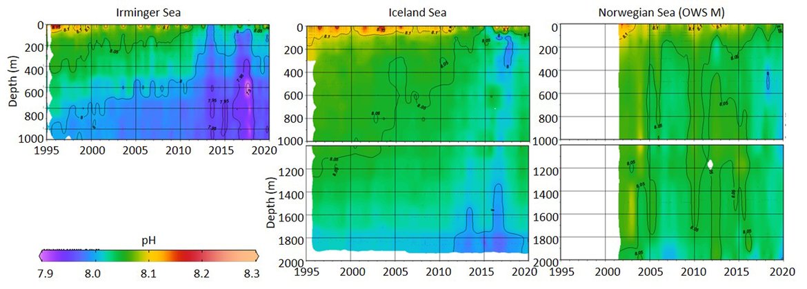
 and aragonite saturation state (ΩArag; bottom panels) at the time series sites Irminger Sea (left), Icelandic Sea (middle), and OWS M in the Norwegian Sea (right) in the Arctic Waters (OSPAR Region I).")
Figure 3.14: Water column pH (top panels) and aragonite saturation state (ΩArag; bottom panels) at the time series sites Irminger Sea (left), Icelandic Sea (middle), and OWS M in the Norwegian Sea (right) in the Arctic Waters (OSPAR Region I).
Furthermore, the GLODAP data product has been used to examine the water column dynamics. GLODAP areas with high data density have been selected (see maps in Figure 3.15) to show the temporal variability in pH and ΩArag over the full water column (Figure 3.15). In the west European Basin, the Iberian Basin, and south of Iceland, the pH and ΩArag are decreasing over time in the ocean interior (Figure 3.15, three upper panel rows), while in the western North Atlantic (Figure 3.15, lower panel row), an increasing pH trend seems to have been mixed further down in the water column, although this result might be an artifact from the sparse temporal resolution.
 are used to determine how pH (left contour plots) and aragonite saturation state (ΩArag; right contour plots) develop over the full water depths and over time. The black lines and dots in the maps show where GLODAP data are collected.")
Figure 3.15: GLODAP data from selected areas (cyan coloured areas in the maps) are used to determine how pH (left contour plots) and aragonite saturation state (ΩArag; right contour plots) develop over the full water depths and over time. The black lines and dots in the maps show where GLODAP data are collected.
The plots in Figure 3.15 illustrate decadal changes in pH and ΩArag, however, the data density is too coarse to infer temporal trends. Soundly quantified trends use data from repeat sections with high-quality CO2 measurements, that have a measurement frequency of less than 5 years over North Atlantic basins such as the Irminger, Iceland, or Eastern North Atlantic (ENA) Basins.
Examining areas with measurement frequencies less than 5 years, show that ocean acidification is occurring along the water column in all basins of the OSPAR Regions except for the deep layers in the East North Atlantic (ENA) Basin below 3 000 m (García-Ibáñez et al., 2016; Vázquez-Rodríguez et al., 2012; García-Ibáñez et al., 2021; Fontela et al., 2020). The reduction in pH in the Irminger Basin (between –0,0018 and –0,0015, Figure 3.16) is faster than in the Iceland Basin (between –0,0016 and –0,0009, Figure 3.16), but in both basins, a significant pH reduction occurs in the bottom waters at approximately 2 500 m. In the ENA Basin, as commented, only significant trends were found down to 2 000 m (between –0,0009 and –0,0008), with magnitudes lower than in the northern basins. The gradual northward increase in ocean acidification rates is associated with the deep circulation of the North Atlantic, where overflow waters from the Greenland-Iceland-Norwegian Seas plunge southwards conveying to depth the signal of their recent contact with the atmosphere. Ocean acidification is mostly associated with the anthropogenic carbon uptake and storage by the ocean, but warming also contributes to decreasing pH in upper waters. At intermediate depths, an intensified remineralization of organic matter, or lack of ventilation reinforces ocean acidification (García-Ibáñez et al., 2016).
Published ΩArag trends in the interior of Irminger and Iceland Seas are of similar range (–0,005 to –0,0014 yr-1) with slightly higher values in the Irminger Sea (Figure 3.16). Opposite to pH trends, the ENA upper and intermediate waters present stronger ΩArag trends than the northern basins (range –0,0080 to –0,0025 yr-1); Figure 3.16). In this sense, the ASH is shoaling at approximately 14, 9 and 7 m yr-1 for the Irminger, Iceland and ENA areas, respectively (García-Ibánez et al., 2021; Fontela et al., 2020). Therefore, intermediate waters will become undersaturated in aragonite much faster in northern waters.
 and aragonite saturation state (ΩArag; right panel) throughout the water column for the Irminger Basin (yellow circles), Iceland Sea Basin (blue squares) and East North Atlantic Basin (ENA; grey triangles)")
Figure 3.16: Published trends for pH (left panel) and aragonite saturation state (ΩArag; right panel) throughout the water column for the Irminger Basin (yellow circles), Iceland Sea Basin (blue squares) and East North Atlantic Basin (ENA; grey triangles)
Numbers in parenthesis represent references: (1) Vázquez-Rodríguez et al. (2012), (2) García-Ibañez et al. (2016), (3) Fontela et al. (2020), (4) García-Ibáñez et al. (2021).
On the continental shelf, and shallow coastal regions of the Greater North Sea, the Celtic Seas, and the Bay of Biscay and Iberian Coast (OSPAR Regions II, III and IV), the surface signal often reaches the seafloor, although this depends on the mixing regime, oceanographic, tidal, and riverine influences. Many of the time series stations reported here for these regions only monitor pH at the near surface, while a few, less frequently monitor the bottom water. As an example, full water column data has been collected at station L4 at WCO since late 2017 (Figure 3.4), and this data shows that there is a seasonal cycle in pH and ΩArag all the way to the bottom waters at 50 m (Figure 3.17). In the upper surface layers, pH and ΩArag increase during the spring and summer phytoplankton blooms which use CO2 to form organic matter. During the spring this higher pH water can still be spread across the water column to the bottom before stratification occurs. During summer, the water becomes stratified separating the high and low pH and ΩArag waters. In the bottom waters, remineralisation of organic matter causes a decrease in pH and ΩArag, and during autumn, this lower pH and ΩArag water is then transferred across the water column when stratification is broken down by storms and mixing events. While this time series is not long enough to show trends throughout the water column, the seasonal dynamics clearly indicate that at present day levels (2018 to 2020), the seasonal decline in ΩArag exposes benthic (bottom-dwelling) organisms to longer periods of lower ΩArag levels (< 2) than surface organisms (Figure 3.17).
 and aragonite saturation state (ΩArag; bottom panel) through water column at WCO L4 station in the Greater North Sea (OSPAR Region II).")
Figure 3.17: Seasonal cycle of pH (top panel) and aragonite saturation state (ΩArag; bottom panel) through water column at WCO L4 station in the Greater North Sea (OSPAR Region II).
Also plotted (grey lines) are in situ density anomaly to indicate seasonal stratification and mixing.
The ERSEM-NEMO model shows annual average trends for pH and ΩArag in the bottom waters between 1990 and 2015 on the shelf region (water depth < 200 m). The rate of pH decline varies across the Greater North Sea, the Celtic Seas, and Bay of Biscay and Iberian Coast (OSPAR Regions II, III, and IV), with some areas experience little or no significant change over the past few decades, and other regions (to the south of Ireland and the northern North Sea) experiencing pH rates down to –0,005 yr-1 (Figure 3.18). Similar patterns are observed in the ΩArag trends (Figure 3.18). The model work highlights that, despite the larger interannual variability observed in these shallow shelf seas, ocean acidification is occurring throughout the water column right down to the bottom waters.
, the Celtic Seas (OSPAR Region III), and the Bay of Biscay and Iberian Coast (OSPAR Region IV) for pH (left panel) and aragonite saturation state (ΩArag; right panel) from NEMO-ERSEM, where water depth < 200 m.")
Figure 3.18: Mean bottom water trends across the Greater North Sea (OSPAR Regions II), the Celtic Seas (OSPAR Region III), and the Bay of Biscay and Iberian Coast (OSPAR Region IV) for pH (left panel) and aragonite saturation state (ΩArag; right panel) from NEMO-ERSEM, where water depth < 200 m.
3.4. Discussion
3.4.1 Time-series observations and their challenges
This report includes data from a variety of time series stations in the OSPAR Regions, and an overview of the different stations is found in Table 3.1 and Supplementary information Table S1 . The concept of time series is multifaceted and one of the few common characteristics is that measurements are collected over time across a very limited spatial area. However, the lengths, sampling frequencies, selected variables, and quality of the time series vary from site to site. In addition, the time series sites are from different areas (e.g., coastal vs. open ocean, or west vs. east of the Mid-Atlantic Ridge) and are therefore influenced by different processes (Figure 3.3;Table 3.2 ). Thus, it is not straight forward to compare the selected data series and some of these challenges are discussed here.
Time-series stations with sampling frequency of less than once per season were excluded from this assessment because these time series do not resolve the seasonal signal, which could bias the trend estimate. Thus, there is no time series data for the large Wider Atlantic (OSPAR Region V) and only a few time series from the Arctic Waters (OSPAR Region I). A further challenge is that when comparing time series, there are often data breaks due to, for example, failure in instrumentation, bad weather, or lack of continued funding. Seasonal biasing of the data might be a particular result of these challenges, which means that, even if the sampling frequency is high, data is mainly collected during one season, for example, in spring and summer when weather conditions tend to be more amenable to sampling. By averaging data into seasonal values, this bias is reduced, and thus makes time series more comparable.
The length of the time series can also alter the confidence in trends; long-term datasets provide more robust assessments of climate-scale trends associated with observing the impacts of ocean acidification caused by the addition of anthropogenic CO2. There are just six time series stations in the OSPAR Regions that are longer than 20 years. Counter to this, these long-term trends dampen out any short-term trends (sub-decadal) that could be associated with changes in other drivers that can mitigate or amplify the ocean acidification signal, as exemplified by Provoost et al. (2010)’s explanations for fluctuations in pH from the Netherlands datasets, and these are also important to understand.
Another challenge is that the quality of different measurements can vary across the time series. This can partly be explained by the lack of high-quality pH instrumentation in the earlier periods of time series, by lack of reference materials for the earliest carbon measurements, and by the evolution of the pH method since approximately 2010 using purified indicators for open ocean high quality measurement. For instance, the early pH data from Belgium and The Netherlands time series was determined using sensor electrodes which had a precision of approximately 0,1, while pH sensors now have a precision of approximately 0,001. Moving forward, since the late 2000s, there has been development of standard protocols, best practise guides, and certified reference materials (CRMs) for monitoring the carbonate system, which all OSPAR parties now follow (e.g., Dickson et al., 2007). In 2021, a new proficiency testing capacity regarding Dissolved Inorganic Carbon (DIC) and Total Alkalinity (TA), organised by QUASIMEME, was introduced across laboratories, and it is highly recommended that all laboratories participate in this. After evaluation of the results and discussion with the participants, further optimisation of the intercalibration exercise will be done in 2022. The quality control issues specific to each dataset are included in Supplementary information Table S.1 and Section S.2.1 .
An important challenge for time series stations, is the lack of sustained funding for long-term time series programs, which hampers the ability to continually collect this important data for climate change monitoring. As highlighted here, long-term data of high quality is needed in order to evaluate longer term trends, especially in complex coastal regions, which could have much shorter influence from other processes alongside the overarching issue of anthropogenic CO2 addition causing ocean acidification. Furthermore, an increased amount of data would pave the way for reduced uncertainty of the reconstructed data products, which require independent validation. Importantly, the time series stations provide critical understanding of the near-shore dynamics, which are often not captured by the wider synthesis products or regional-scale modelling. In terms of interactions with humans, these near-shore environments are arguably of most significance as they are often the locations of human marine activity, for instance aquaculture, fishing, industry, tourism, and shipping. As demonstrated by this assessment, without time series networks such as those in France, Belgium and The Netherlands, these higher rates of change in pH would not be observed and therefore could not be explored to understand the drivers. This lack of understanding in turn prevents scientists from providing evidence and advice on mitigation and adaptation policies as a result of climate change (e.g., impacts, risk assessment, environmental status assessments, adaptation planning).
Despite the challenges mentioned above, most of the stations included in this report show negative trends in pH and ΩArag since observations began in the early 1980s (Figure 3.2;Table 3.1 ). Rates vary significantly across the OSPAR Regions, with highest rates occurring in the very near-shore stations in the Greater North Sea, the Celtic Seas, and the Bay of Biscay and Iberian Coast (OSPAR Regions II, III and IV).
3.4.2 GLODAP data product and its challenges
The Global Ocean Data Analysis Project (GLODAP) data product has been used here to illustrate variability in pH and ΩArag in the ocean interior of selected areas of the OSPAR Regions. The GLODAP data product aims at collecting carbon, tracers and ancillary hydrography and biogeochemical data from cruises covering full depth across the ocean interior over the last 50 years or so. GLODAP compiles the data in a user-friendly and ready to use common format, with strict quality control procedures implemented to avoid biases in the data. The amount of data is enormous, however, when focusing in on specific ocean areas it becomes apparent that the spatial and temporal resolution often is too coarse to, with confidence, determine trends in ocean acidification over areas like the OSPAR Regions and in particular for the surface waters (< 25 m). There are, for example, more summer data than winter data which would bias annual surface averages. However, since there is less variability in the ocean interior, estimates of pH and ΩArag trends based on GLODAP data product have less uncertainty compared to GLODAP derived trends in the surface ocean.
Sustaining repeat hydrographic cruises following the GO-SHIP recommendations is crucial, not only to document ocean acidification changes but to understand the drivers. The carbon system and its interaction with the multiple consequences of climate change in the ocean (including warming, increased stratification, circulation changes) is complex; for example, climate change feedbacks could mitigate (higher salinity induces higher alkalinity and higher buffer capacity) or intensify (reduced ventilation induces a higher rate of remineralisation and lowers the buffer capacity) chemical changes in the deep ocean. These sort of data products are relied upon by the reconstruction and modelling communities to understand the processes, provide high quality data for statistical modelling, and critically for validation. They also provide the large-scale context in which the local scale in situ observations can be set and evaluated.
3.4.3 Challenges for reconstruction synthesis and modelling products
This review includes data from both reconstruction synthesis products and process-based modelling. The reconstruction synthesis products are only available for the surface and rely on good quality data being available to provide the statistical training that is used to create them (e.g., SOCAT pCO2 data, World Ocean Atlas (WOA) data for temperature and salinity, and data that is used to derive alkalinity-salinity relationships). As highlighted for the GLODAP data product, although over ocean scales large amounts of data exist, when scaling down to regions and through time, clearly these observational data are not evenly distributed. This data discrepancy will ultimately lead to bias within synthesis and modelling products which rely on them, not only for generating the models but also for validation. Models are only as good as the understanding of the processes built into them, and furthermore, the model results will always be a trade-off between spatial scale, complexity of processes, and costs. Overall, the reconstruction synthesis products showed similar results to each other and to the process-based modelling (Figure 3.2;Table 3.1 ). However, in the shelf-sea regions, especially close to the coast the products were not able to capture the large dynamics, nor the longer-term trends observed at the time series stations.
Regional synthesis mapping exercises have been carried out for shelf regions, for instance, Becker et al. (2021) used a newly developed mapping technique together with observations to estimate pH trends in the North Sea and other coastal areas over the period 1998 to 2016. Their pH trend in the North Sea was on average –0,0015 yr-1, ranging from approximately –0,003 yr-1 along the east coast of the United Kingdom to –0,0005 yr-1 along the west coast of Denmark. Regionally this matches well with both global synthesis products describe here, however, this latter rate is still an order of magnitude lower than rates obtained from the Dutch stations in the North Sea when compared over the same period (1998 to 2016: -0,005 to –0,006 yr-1). This discrepancy could be explained by uncertainties in the developed mapping technique, which is based on a limited amount of data in the North Sea over longer periods of time. Additionally, many of these techniques rely on alkalinity-salinity relationships, which tend to break down near shore (e.g. Carstensen and Duarte, 2019). Enhanced understanding of the processes and drivers in the coastal region is therefore needed to improve both reconstruction synthesis products and modelling efforts.
3.4.4 Comparison of the different evidence lines
There are many differences between data types: in situ data, synthesis reconstruction, and modelling products, which include scale (Figure 3.1), processes, calculated vs measured variables, and many others. These differences make it difficult to accurately compare these data types and as such, no attempt to directly compare absolute values was made. This issue is highlighted by Figure 3.19, which illustrates that there may not appear to be a good match between some time series datasets and some synthesis products (in this example, CMEMS-LCSE-FFNN; Figure 3.19 left panel). However, when only the time series stations that match the synthesis product on temporal scales and in location are included (Figure 3.19 right panel), there is clearly good corroboration between these different data types.

Figure 3.19: Maps of surface pH trend from CMEMS-LCSE-FFNN, with time series stations overlaid with the associated colour representing the trend.
Left panel includes all time series station that displayed a significant trend, middle panels include only time series stations that had significant trends and were longer than 10 years, right panel shows only time series stations that were longer than 10 years, had significant trends, and overlapped with the regional coverage of the synthesis product.
The differences between the data types are also highlighted when exploring the average variability that a region experiences. For the purposes of this assessment, only average range across the seasons is reported. The seasonal variability found in the synthesis reconstruction products was representative of the seasonal variability expected for open ocean systems reflecting the simpler dynamics of warming, cooling, photosynthesis and respiration. Clearly, more drivers are at play within the coastal and near-shore areas in the Greater North Sea, the Celtic Seas, and the Bay of Biscay and Iberian Coast (OSPAR Regions II, III and IV), as evidenced from the in situ time series data (Figure 3.20; Figure 3.3;Table 3.2 ). The process-based regional model was able to capture more of the seasonal dynamics associated with these shelf environments (Figure 3.20).
While there exists a clear association with increased levels of variability and distance offshore (Figure 3.20), this is not a controlling driver. It is a proxy for the differing processes associated with near-shore environments. Within this boundary, proximity to rivers, habitat types, sediment types and even geology can and will influence the natural seasonal dynamics, with human interactions adding to these (Figure 3.3;Table 3.2 ).
Figure 3.20: Mean seasonal range of pH (top box) and aragonite saturation state (ΩArag; bottom box) for in situ time series stations (red), OceanSODA-ETHZ reconstruction synthesis product (green), CMEMS-LCSE-FFNN reconstruction synthesis product (yellow), and model NEMO-ERSEM (blue) across each OSPAR Region (I = Arctic Waters; II = The Greater North Sea; III = The Celtic Seas; IV = Bay of Biscay and Iberian Coast; V = Wider Atlantic).
3.5 Concluding remarks and recommendations
Ocean acidification is occurring across all OSPAR Regions, such that it is observable in terms of decreasing seawater pH and aragonite saturation state (ΩArag) over decadal time-periods. The rates of ocean acidification vary from region to region, with strongest rates of decline apparent in the near-shore and coastal regions. The near-shore is influenced by factors that amplify the impacts of ocean acidification resulting from anthropogenic CO2 addition. Some factors include changes in: oceanographic properties, such as temperature, salinity and mixing dynamics; acidic compound additions, such as sulphur; river run-off; precipitation; land-use; sediment-water interactions; and / or biological processes. These factors also result in increased short-term variability, both on seasonal and interannual time-scales.
Not only is ocean acidification impacting surface waters, due to ocean mixing processes it is penetrating into the deep ocean. Deep-water in situ ocean time series sites provide evidence of shoaling of the aragonite saturation horizon (ASH), while shallow-water coastal sites demonstrate seasonally lower pH and aragonite saturation conditions in the bottom waters.
Reconstruction synthesis products (both global and regional level) and process-based modelling efforts overall show consistent trends with declining pH and aragonite saturation state. However, they presently do not capture these very near-shore dynamics associated with many of the coastal time series stations in the OSPAR Regions, especially in the Greater North Sea (OSPAR Region II), the Celtic Seas (OSPAR Region III) and the Bay of Biscay and Iberian Coast (OSPAR Region IV).
A number of recommendations have been mentioned throughout this section and are highlighted here:
- While there are increasing numbers of high-quality long-term time series stations, there is a need for Contracting Parties to provide continued support to sustain these and build on them, as well as recognise their importance.
- Time-series stations need to be monitoring more than one variable of the carbonate system (i.e., not just pH) together with associated data, in order to fully elucidate the carbonate system, including aragonite saturation state, and investigate the drivers of change.
- Near-shore and shallow coastal environments must be monitored at much higher spatial and temporal resolution than the open ocean in order to understand the drivers occurring alongside the anthropogenic increase in CO2, and to project biological response.
- Time-series stations need to continue with strong quality assurance (QUASIMEME, CRMs, and others) and follow standard operating procedures and guide for best practices. Further, all monitoring laboratories should be involved in the Global Ocean Acidification Observing Network (GOA-ON) to keep up-to-date with quality control efforts as well as feedback and develop these.
- Monitoring of ocean acidification and biological responses should be coupled to support the assessment of ecosystem risk and consequences, and better inform management strategies.
- The data availability and transparency should be improved in order to increase data flow between data centres, so that data can be incorporated into synthesis products and reports, while still acknowledging and maintaining connection with the original data collectors.
- Down-scaled process-based models for the near-shore and coastal environment need to be utilised in order to understand and predict the dynamics of ocean acidification in these areas.
4. Projections of Future Ocean Acidification
Key messages
- Ocean acidification in OSPAR Regions I to IV is projected for the period up to 2050 using two regional models and two emissions scenarios (high and mid).
- Ocean acidification is projected to occur in all four OSPAR Regions, and stronger acidification is projected with higher emission scenarios.
- In the higher emission scenario used, ocean acidification is projected to even accelerate towards the end of this century.
- The projected trends of ocean acidification are spatially very variable. For example, in the Arctic region, surface pH trends range from –0,007 yr-1 near the North Pole to close to 0 in few areas, like the edge of the sea-ice. In the other regions, the range is smaller (-0,004 to -0,002 yr-1) but still significant.
- Part of the seafloor is projected to be corrosive to exposed calcareous structures:
a. In the European shelf, in the mid-emission scenario, this condition will be seasonal and only occurring in a small region, but it will impact a large part of the seafloor in the high emission scenario by 2100;
b. The deep arctic basin is projected to be already corrosive to exposed calcareous structures, and in the high emission scenario this area is projected to double.
- Using multiple regional models (ensembles) will reduce the uncertainty and increase the robustness of the presented projections.
4.1 Introduction
Coupled hydrodynamic-biogeochemical models are numerical representations of the marine environment that are able to simulate its behaviour under specific forcing. They are able to describe the physical properties of the water column (e.g., temperature, salinity, currents), its chemical composition (e.g., oxygen, various nutrients, the carbon concentration, pH) and some aspects of the biological elements (e.g., phytoplankton, zooplankton, bacteria).
These models are powerful tools to better understand the dynamics of complex systems such as the marine environment, and they can provide comprehensive information on current state and trends that is impossible to achieve through observations. They are also the only tool available to make projections of the future state of the marine environment depending on different emission scenarios. Earth System Models (ESM) – implemented in the Coupled Model Intercomparison Project (CMIP) and used by IPCC in their comprehensive Assessment Report of climate change – use coupled hydrodynamic-biogeochemical models to represent how the oceans influence the climate and how they respond to climate change.
Because of computational constraints, oceans in ESM are represented with a relatively coarse horizontal resolution, usually around 1 degree (approximately 60 to 100 km), and with a very simple ecosystem structure. Therefore, the small-scale variability typically occurring in the highly dynamic and complex environments found in many parts of the OSPAR Maritime Area is not well represented by such large-scale models. To fill this gap, higher resolution regional models are usually implemented: given the smaller regional domain included in these models, they can afford a higher resolution (generally below 10 km) and are therefore more suited to represent what happens in shelf seas and coastal areas.
All such coupled models are based on the same key marine ecosystems processes, however some of the simplifying assumptions behind them differ among models and so is the level of detail with which specific processes are represented. This is an inevitable consequence of the complexity of the marine environment, and it is required to find a balance between the need for realism and the computational constraints. Some typical differences between biogeochemical models are the structure of the planktonic food web (varying from one group per trophic level to few dozen for the more complex models) and the elemental composition of plankton (that can be fixed or variable). As a consequence of such variability in model assumptions and structure, the projections that marine models can provide to the same change in the external environment may differ, producing uncertainty in those projections. Combining models and observations can help in assessing and reducing the uncertainty in each of them, and so is running ensemble (collection) of different models under the same condition to then look at the envelope of the plausible responses and to ascertain what is the more likely response. This approach is commonly used in the IPCC comprehensive Assessment Report, where more than 30 models were run to provide the range of the potential response in the various scenarios.
Here outputs from two different regional models covering two different areas within the OSPAR Maritime Area are used (Figure 4.1).

Figure 4.1: bathymetry of the two model domains.
On the left, the domain used to represent the Arctic region (NOREWCOM.E2E; OSPAR Region I) and on the right the one used for the regions of the Greater North Sea, Celtic Seas and the Bay of Biscay and Iberian Coast (AMM7; OSPAR Regions II, III and IV). Pink lines highlight the limits of OSPAR Regions as included in the models.
The NORWegian ECOlogical Model system End-To-End (NORWECOM.E2E) is a regional coupled physical, chemical, biological model system (Skogen et al., 1995) originally developed to study primary production, nutrient budgets, and dispersion of particles such as fish larvae and pollution. It has been extended with a module to project ocean acidification (Skogen et al., 2014; 2018). Here it has been used for the Nordic Seas to project the trends of pH and ΩArag for the Arctic (OSPAR Region I).
The model spans a domain covering the whole Nordic Seas, the Barents Sea, and parts of the Arctic from approximately 60°N (Figure 4.1). The model is run in offline mode with downscaled physics from the NorESM2 global climate model under CMIP6 emission scenarios using the NEMO model. The horizontal resolution is approximately 10 km.
The AMM7 (short for Atlantic Margin Model at 7 km) is based on the ocean dynamic model NEMO (Nucleus for European Modelling of the Ocean, Madec, and the NEMO team, 2016) and ERSEM (Butenschön et al., 2016), a biogeochemical model that describes the cycling of the major elements (carbon, nitrogen, phosphorus and silicate) across the planktonic food web and its effect on the dynamics of the carbonate system.
The AMM7 domain spans from 40° N to 65° N and from 20° W to 12° E (Figure 4.1). It has a horizontal resolution of approximately 7 km and a vertical resolution of 51 levels, meaning that the water column is subdivided in 51 layers, thinner on the shelf where the water column is shallower, and thicker in the open ocean, especially close to the seafloor.
This model has been used to provide both recent trends of ocean acidification (hindcast mode – results are shown in Section 3.2.3) and future trends (projection mode).
In the projection mode, the model is forced using atmospheric climate projections (2015-2050) from the CMIP5 model Hadley Global Environment Model 2 – Earth System (HadGEM2-ES, Jones et al., 2011) as downscaled in the Coordinated Regional Downscaling Experiment (CORDEX) program by the SMHI-RCA4 regional climate model (Strandberg et al., 2014) developed by the Swedish Meteorological and Hydrological Institute (SMHI). The use of downscaled atmospheric projections allows for a better description of regional and local dynamics thanks to the higher resolution (approximately 10 km) compared to the coarse resolution in HadGEM2-ES (> 100 km). The open ocean boundary conditions are taken directly from the ocean component of HadGEM2-ES.
In order to extend the analysis to 2100 in the AMM7 region, an additional simulation was used, where atmospheric forcing and open ocean boundary condition comes directly from the CMIP5 model IPSL-CM5-MR (Dufresne et al., 2013). The climate sensitivity of IPSL-CM5-MR is similar to that one of HadGEM2-E and therefore the uncertainty introduced by merging simulations driven by two different models is limited and does not alter the conclusions drawn in the report.
4.2 Future Projections
The two regional models have been used to represent different scenarios of ocean acidification to forecast future trends in pH and ΩArag. The main temporal horizon used is the mid-century (approximately 2050) to focus on the more immediate risks, however some consideration on the longer time (approximately 2100) will also be provided to offer some insight to the further impact that the OSPAR Maritime Area could experience for two selected emission scenarios: a mid- emission scenario and a high emission scenario.
In the context of the latest IPCC Assessment Report (AR6), several potential future scenarios have been defined (Figure 4.2), based on Shared Socio-economic Pathways (SSP) and Representative Concentration Pathways (RCP). SSPs represent different pathways of development for the society and the economy, that have been summarised in 5 different narratives: “sustainability” (or SSP1), “middle of the road” (SSP2), “regional rivalry” (SSP3), “inequality” (SSP4) and “fossil fuelled development” (SSP5). RCPs instead represent the evolution of greenhouse gas emissions and concentration in the atmosphere that determine a total radiative forcing by the year 2100 (i.e. the energy flux in the atmosphere causing climate change) varying from 1.9 W m-2 to 8.5 W m-2, with various intermediate scenarios. In the previous Assessment Report (AR5), future scenarios were only defined by the RCP (2.6, 4.5, 6.0 and 8.5), assuming that there was only one possible pathway for society to develop each specific pathway of emission and concentration.
The combination of SSP and RCP (e.g. SSP5-8.5 means a “fossil fuelled development” scenario that would cause an increase in radiative forcing to 8.5 W m-2 by 2100) provides a wide range of scenarios, that potentially allow to explore more future projections. Due to the high cost of running Earth System Models (ESM) in multiple scenarios, two sets of scenarios were prioritised (called tier 1 and tier 2, see Figure 4.2): all the research centres contributing to CMIP6 were compelled to run all scenarios part of tier 1, while tier 2 scenarios were optional. As a consequence, if the focus is only on tier 1 and tier 2 scenarios, even in the new context of SSPs and RCPs, there is an almost unique correspondence between emission and concentration scenarios and socio-economic pathways (with the exception of RCP3.4 that could be achieved either under an “inequality” narrative as well as in an overshoot “fossil fuelled development” narrative in which the emissions initially increase considerably and then are subsequently reduced to limit climate change).
Finally, it is important to note that, despite giving the same radiative forcing, equivalent RCP in the two cycles of the assessment reports, are not identical in term of emissions and concentration of greenhouse gases (Wyser et al., 2020).
. Tier 1 and tier 2 represent the scenarios that have been prioritised in running Earth System Models (ESM), with only tier 1 being compulsory to participate to the intercomparison project (reproduced from O’Neill et al., 2016, CC by 3.0).")
Figure 4.2: matrix of SSP and RCP scenario compared to the previous RCP based scenario (green boxes). Tier 1 and tier 2 represent the scenarios that have been prioritised in running Earth System Models (ESM), with only tier 1 being compulsory to participate to the intercomparison project (reproduced from O’Neill et al., 2016, CC by 3.0).
The RCPs considered here are RCP 8.5, and RCP 4.5. The first one is a high emission pathway, that assumes that the concentration of greenhouse gases will increase considerably during this century to cause an increase in the radiative forcing by the end of the century of 8.5 W m-2. Even though this can be seen as a worst-case scenario, where emissions of greenhouse gases increase significantly, it is in close agreement with the historical trend of CO2 cumulative emissions and it is close to the cumulative CO2 emissions by 2050 considering the pledges made by several countries before the recent net-zeros commitments (Schwalm et al., 2020). For this reason, it is still useful to consider this scenario as an indication of what could realistically happen by mid-century if all pledges are not met.
RCP4.5 is an intermediate stabilisation pathway that assumes an increase in the radiative forcing of 4.5 W m-2 by 2100, corresponding to an intermediate emission scenario. It assumes a peak in emission of CO2 from fossil fuel between 2040 and 2050 and then a decrease of CO2 emission and a stabilisation of the other greenhouse gases. This scenario does not meet the goal of the Paris Agreement, but it considers a stabilisation of emissions where mild mitigation measures are implemented. It is also the second closest scenario to the cumulative CO2 emissions by 2050 (Schwalm et al., 2020). It is important to highlight that while NORWECOM.E2E has been forced with CMIP6 results (i.e., SSP5-8.5 and SSP2-4.5), NEMO-ERSEM has used CMIP5 outputs (i.e., RCP8.5 and RCP4.5). Consequently, while the climate scenarios simulated in both models are equivalent, the atmospheric concentration of CO2 is not the same with potential consequences on the rate of ocean acidification (see Section 4.5)
4.3 Projected trends
In the following sections, the trend of pH and ΩArag for surface waters and for waters close to the seafloor will be presented. These trends have been calculated as the slope of the linear regression of the annual mean value of the variable in each grid cell of the domain. It is important to highlight that while NORWECOM.E2E has been forced with CMIP6 results (i.e., SSP5-8.5 and SSP2-4.5), NEMO-ERSEM has used CMIP5 outputs (i.e., RCP8.5 and RCP4.5). Consequently, while the climate scenarios simulated in both models are equivalent, the atmospheric concentration of CO2 is not the same with potential consequences on the rate of ocean acidification (see Section 4.5).
4.3.1 Surface trends
Table 4.1 summarises average trends of pH and ΩArag for the OSPAR Regions and the within region variability. The average projected trends for pH compare well with current observed trends from synthesis products (see Figure 3.2).
| OSPAR Region | Variable | SSP2-4.5 / RCP 4.5 | SSP5-8.5 / RCP 8.5 |
|---|---|---|---|
| I Arctic Waters | pH | -0,0017 yr-1 (0,0001 to -0,0070) | -0,0021 yr-1 (0,0002 to -0,0065) |
| ΩArag | -0,0042 yr-1 (0,0017 to -0,0137) | -0,0055 yr-1 (0,0014 to -0,0137) | |
| II Greater North Sea | pH | -0,0023 yr-1 (-0,0016 to -0,0029) | -0,0036 yr-1 (-0,0026 to -0,0042) |
| ΩArag | -0,0093 yr-1 (-0,0060 to -0,0128) | -0,0156 yr-1 (-0,0117 to -0,0199) | |
| III Celtic Seas | pH | -0,0021 yr-1 (-0,0016 to -0,0026) | -0,0033 yr-1 (-0,0029 to -0,0036) |
| ΩArag | -0,0082 yr-1 (-0,0049 to -0,0112) | -0,0134 yr-1 (-0,0105 to -0,0161) | |
| IV Bay of Biscay and Iberian Coast | pH | -0,0023 yr-1 (-0,0018 to -0,0028) | -0,0035 yr-1 (-0,0029 to -0,0041) |
| ΩArag | -0,0110 yr-1 (-0,0068 to -0,0135) | -0,0167 yr-1 (-0,0130 to -0,0198) |
Arctic Waters (OSPAR Region I)
The average trend of pH in this region projected by NORWECOM.E2E is -0,0017 yr-1 under the SSP2-4.5 scenario and -0,0021 yr-1 under SSP5-8.5, an increase of 24% in the trend between the two scenarios (Figure 4.3). The spatial variability is very high: the presently ice-covered area closer to the pole experiences a much stronger acidification with a trend steeper than -0,021 yr-1 in SSP2-4.5 (and –0,018 yr-1 under SSP5-8.5) while the area close to the sea-ice edge shows a slight increase of pH. There is a general stronger decline in the Barents Sea than in the Nordic Seas and an east / west gradient with a higher trend towards the east.
The spatial patterns of trends of ΩArag are similar to those seen for the pH with the highest change in the ice-covered areas around the pole where the model is simulating undersaturation, even at present day, a stronger decline in the Barents Sea than for the Nordic Seas, and an east / west gradient. On average the trend is 30% stronger in the SSP5-8.5 emission scenario compared to that of SSP2-4.5 (-0,0055 and -0,0042 yr-1, respectively). In 2050 the model projects that the surface water could be corrosive for some calcium carbonate structures in the Arctic north of the Fram Strait, in the north-eastern Barents Sea (close to Novaya Zemlya), and in a slight band along the Norwegian coast under the SSP5-8.5 emission scenario.
 and ΩArag (bottom; yr-1) between 2015 and 2049 as projected by the NORWECOM model under the SSP2-4.5 scenario (left) and SSP5-8.5 scenario (right). Only data within the OSPAR Regions has been shown.")
Figure 4.3: Trend of surface pH (top; yr-1) and ΩArag (bottom; yr-1) between 2015 and 2049 as projected by the NORWECOM model under the SSP2-4.5 scenario (left) and SSP5-8.5 scenario (right). Only data within the OSPAR Regions has been shown.
Greater North Sea (OSPAR Region II)
The average trend of surface pH in this region is -0,0023 yr-1 in the RCP4.5 scenario and -0,0036 yr-1 in RCP8.5 (Figure 4.4). Compared to the Arctic region, the spatial variability of the trends is smaller but still relevant: 90% of region II has been projected to experience a trend in surface pH varying between –0,0016 yr-1 and –0,0029 yr-1 under RCP4.5, and between -0,0026 yr-1 and -0,0042 yr-1 under RCP8.5. This high variability could lead to ocean acidification impacting various areas of the region differently, with the central North Sea potentially more impacted than the Southern coastal area.
This variability is driven by several factors like land-ocean interactions (e.g., some of the big river from continental Europe discharging in the Southern North Sea have high alkalinity and therefore increase the buffer capacity in this coastal area), different level of productivity in the areas (higher productivity can lead to higher maximum pH during the bloom) and different mixing pathways among water masses.
The range of the pH seasonal cycle in the area can be as high as 0,7 (especially in coastal areas), generally larger than the ocean acidification signal in the 50 years considered here. A higher amplitude of the seasonal cycle might imply a higher resilience to ocean acidification of the organism living in this environment because they are already adapted to change (see Section 5.3). At the same time, higher variability might lead to higher likelihood of passing critical thresholds even if for short period, with higher risk of acute effect on organisms.
The average trends of ΩArag in this region are -0,0093 yr-1 and -0,0156 yr-1 with a spatial variability that is similar to the one projected for pH.
 and ΩArag (bottom; yr-1) between 2000 and 2050 as projected by the AMM7-NEMO-ERSEM model under the RCP 4.5 scenario (left) and RCP8.5 scenario (right). Only data within the OSPAR Regions has been shown.")
Figure 4.4: Trend of surface pH (top; yr-1) and ΩArag (bottom; yr-1) between 2000 and 2050 as projected by the AMM7-NEMO-ERSEM model under the RCP 4.5 scenario (left) and RCP8.5 scenario (right). Only data within the OSPAR Regions has been shown.
Celtic Seas (OSPAR Region III)
The average trends of surface pH in this region are -0,0021 yr-1 (RCP4.5) and -0,0033 yr-1 (RCP8.5), while those for ΩArag are -0,0082 yr-1 (RCP4.5) and -0,0134 yr-1 (RCP8.5). The range of spatial variability is similar to the one for the Greater North Sea, with the coastal area showing the smaller trend (Figure 4.4).
Bay of Biscay and Iberian Coast (OSPAR Region IV)
The average trends of surface pH in this region are -0,0023 yr-1 (RCP4.5) and -0,0035 yr-1 (RCP8.5), while those for ΩArag are -0,0110 yr-1 (RCP4.5) and -0,0167 yr-1 (RCP8.5). The lowest trends are projected to be along the Iberian coast and along the shelf break in the middle of the Bay of Biscay (Figure 4.4). On the contrary, trends of ΩArag in the open part of the Bay of Biscay are the strongest, especially in the RCP8.5 scenario.
4.3.2 Seafloor trends
Table 4.2 summarises the trends of pH and ΩArag in the waters above the seafloor. Due to the way the different models describe the vertical resolution, the bottom water values projected by the models are representative of the values from one or few meters above the seafloor in the shallow areas to several dozens of meters in the deeper areas.
Furthermore, for ocean acidification trends in bottom waters of the Greater North Sea, the Celtic Seas, and the Bay of Biscay and Iberian Coast (OSPAR Region II, III and IV), the focus is only on the areas that are within the European Shelf, i.e. where the bathymetry is shallower than 200 m. In the current model configuration, estimates of the carbonate system provided by this model in the deeper ocean are indeed less reliable due to the way Total Alkalinity is treated in the model (Artioli et al., 2012).
| OSPAR Region (as represented in the model domain) | Variable | SSP2-4.5 / RCP4.5 | SSP5-8.5 / RCP8.5 |
|---|---|---|---|
| I Arctic Waters | pH | -0,0008 yr-1 (0,0007 to -0,0021) | -0,0010 yr-1 (0,0008 to -0,0024) |
| ΩArag | -0,0020 yr-1 (0,0013 to -0,0051) | -0,0026 yr-1 (0,0013 to -0,0066) | |
| II Greater North Sea | pH | -0,0027 yr-1 (-0,0020 to -0,0033) | -0,0040 yr-1 (-0,0033 to -0,0048) |
| ΩArag | -0,0100 yr-1 (-0,0068 to -0,0123) | -0,0145 yr-1 (-0,0121 to -0,0177) | |
| III Celtic Seas | pH | -0,0022 yr-1 (-0,0014 to -0,0031) | -0,0034 yr-1 (-0,0031 to -0,0039) |
| ΩArag | -0,0076 yr-1 (-0,0033 to -0,0120) | -0,0122 yr-1 (-0,0096 to -0,0153) | |
| IV Bay of Biscay and Iberian Coast | pH | -0,0018 yr-1 (-0,0013 to -0,0021) | -0,0037 yr-1 (-0,0030 to -0,0044) |
| ΩArag | -0,0054 yr-1 (-0,0032 to -0,0077) | -0,0137 yr-1 (-0,0113 to -0,0175) |
Arctic Waters (OSPAR Region I)
The average projected trend of bottom water pH for Arctic Waters (OSPAR Region I) are -0,0008 yr-1 under SSP2-4.5 and -0,0010 yr-1 under SSP5-8.5, an increase of 30% in the trend between the two scenarios (Figure 4.5). The range of spatial variability is high although lower than those projected for the surface. The spatial pattern of trends is also very different compared to the surface one, largely reflecting the large difference in bottom depths: the deep region of the Arctic and the deeper parts of the Nordic Seas show the smallest trend, with values that can be close to zero. On the contrary, the shallower Barents Sea and along the Greenland and Norwegian shelves show higher trends, however still much lower than those projected for the surface.
The average projected trends of bottom water ΩArag are: -0,0020 yr-1 and -0,0026 yr-1 for the SSP2-4.5 and SSP5-8.5 scenarios, respectively. The spatial patterns are similar to those seen for the pH with the highest change in the shallow parts of the area (Barents Sea, Greenland and Norwegian shelfs) and a much slower change in the deep parts (Arctic and Nordic Seas).
 and ΩArag (bottom; yr-1) between 2015 and 2049 as projected by NORWECOM.E2E under the SSP2-4.5 scenario (left) and SSP5-8.5 scenario (right) in the Arctic Waters (OSPAR Region I). Only data within the OSPAR Region has been shown.")
Figure 4.5: The trend of bottom waters pH (top; yr-1) and ΩArag (bottom; yr-1) between 2015 and 2049 as projected by NORWECOM.E2E under the SSP2-4.5 scenario (left) and SSP5-8.5 scenario (right) in the Arctic Waters (OSPAR Region I). Only data within the OSPAR Region has been shown.
Greater North Sea (OSPAR Region II)
In the Greater North Sea (OSPAR Region II), water above the seabed experiences a seasonal acidification in the summer and early autumn period even in present day due to natural processes. During this season, surface waters warm up faster than the rest of the water column and therefore becoming lighter: if the water column is deep enough (usually more than 30 m) and currents are not particularly strong, then the water column stratifies with a lighter surface layer that is free to exchange CO2 with the atmosphere, and a deeper denser layer where CO2 can only be exchanged horizontally. During this period, bottom waters also receive a significant amount of organic matter from the decay of the phytoplankton blooms occurring during spring and summer. The organic matter stimulates the growth of various heterotrophic organisms (bacteria, zooplankton, and benthic fauna): while consuming all the organic matter they produce CO2 through respiration, that, due to the stratification, accumulates in the bottom waters. As for atmospheric CO2, the increase of CO2 causes an acidification of bottom waters that disappears in late autumn and winter when the water column cools down and becomes fully mixed again: in these conditions the accumulated CO2 is released to the atmosphere.
Under present conditions, the seasonal acidification does not lead to significant impact, as this is within the natural variability. Under future scenarios however, the seasonal process can exacerbate the global ocean acidification trends in part of these areas leading to steeper trends in pH and ΩArag.
The average trends of pH in bottom waters in the Greater North Sea are -0,0027 yr-1 in the RCP4.5 scenario and -0,0040 in the RCP8.5, between 10% and 15% steeper than at surface (Figure 4.6). This difference is particularly evident in the central and northern part of the North Sea where stratification is more important.
The average trends of ΩArag are -0,0100 yr-1 and -0,0145 yr-1 and the spatial pattern is similar to the one of pH, with steeper trends in the Northern North Sea and close to the shelf break.
Celtic Seas (OSPAR Region III)
Due to the generally shallower bathymetry of the Celtic Seas compared to the Greater North Sea, this area is less impacted by the seasonal acidification, and the bottom water trends are indeed closer to those shown at the surface. For pH these are -0,0022 yr-1 and -0,0034 yr-1 for RCP4.5 and RCP8.5 respectively and -0,0076 yr-1 and -0,0122 yr-1 for ΩArag (Figure 4.6). Trends are lower in the coastal region and stronger close to the shelf break.
In particular, under the RCP4.5 scenario part of the Celtic Seas is projected to experience minimal acidification, even lower than the surface trend and this is because the model projects this area as a lower pH area.
Bay of Biscay and Iberian coast (OSPAR Region IV)
The pH trends in the bottom water of this region are -0,0018 yr-1 (in RCP4.5) and -0,0037 yr-1 (in RCP8.5), while for the ΩArag these are -0,0054 yr-1 and -0,0137 yr-1 (Figure 4.6). It is important to note that only a small fraction of the bottom waters of this region belong to the shelf and are therefore considered in this analysis. Similarly, to what has been projected for the deeper part of the Arctic, trends in the deep part of the Bay of Biscay and of the North East Atlantic are expected to be very small given their distance from the surface.
 and ΩArag (bottom; yr-1) between 2015 and 2049 as projected by the AMM7-NEMO-ERSEM model under the RCP4.5 scenario (left) and RCP8.5 scenario (right) on the North Western shelf. Only data within the OSPAR Regions has been shown.")
Figure 4.6: The trend of bottom water pH (top; yr-1) and ΩArag (bottom; yr-1) between 2015 and 2049 as projected by the AMM7-NEMO-ERSEM model under the RCP4.5 scenario (left) and RCP8.5 scenario (right) on the North Western shelf. Only data within the OSPAR Regions has been shown.
4.4 Projections beyond 2050
In this report, the main temporal horizon considered for the projection is 2050. However, it is important to consider also what are the changes that models project beyond 2050 towards the end of the century. It is indeed after 2050 that the different scenarios diverge more significantly, and in the highest emission scenario the rate of acidification accelerates (Figure 4.7).
")
Figure 4.7: The global ocean surface pH as projected by the CMIP6 ensemble of Earth System Models (ESM)
(Figure SPM.8, Panel (c) from IPCC, 2021: Summary for Policymakers. In: Climate Change 2021: The Physical Science Basis. Contribution of Working Group I to the Sixth Assessment Report of the Intergovernmental Panel on Climate Change [Masson-Delmotte, V., P. Zhai, A. Pirani, S.L. Connors, C. Péan, S. Berger, N. Caud, Y. Chen, L. Goldfarb, M.I. Gomis, M. Huang, K. Leitzell, E. Lonnoy, J.B.R. Matthews, T.K. Maycock, T. Waterfield, O. Yelekçi, R. Yu, and B. Zhou (eds.)]. Cambridge University Press, Cambridge, United Kingdom and New York, NY, USA, pp. 3−32, doi:10.1017/9781009157896.001.)
In this section, projections up to 2100 of ΩArag in the waters above the seafloor are shown. The divergence between scenarios will be assessed comparing projections in the Arctic region only, because unfortunately no simulations of RCP4.5 up to 2100 were available for the AMM7 NEMO-ERSEM model. Both models are used, however, to show how ocean acidification is projected to accelerate in the RCP8.5 emission scenario after 2050. In particular, the focus will be on the extension of the undersaturated area, i.e., the area of the seafloor that is projected to be covered by waters with a value of ΩArag below 1. The value of 1 is a chemical threshold that separates corrosive or undersaturated conditions, where existing and exposed carbonate structures made of aragonite will start to dissolve (ΩArag is below 1), and oversaturated condition (ΩArag is higher than 1), where existing carbonate structures are safe and more aragonite can be formed in the water through purely chemical processes. It is important to note that this is purely a chemical threshold, and it is less relevant for organisms and their ability to calcify. As explained in Section 5.3, organisms can adapt to live (and calcify) in acidified region, therefore the expansion of the undersaturated area does not imply the collapse of all calcifying species, but it highlights a further threat they will be exposed to.
Arctic Waters (OSPAR Region I)
In the SSP2-4.5 scenario, the model projects that approximately 18% of the seafloor of the Arctic Waters (or 1 million km2, Figure 4.8) is currently already covered by undersaturated water and by 2050 this will only marginally increase to just under 20% (or 1.1 million km2). The undersaturated areas correspond to the deepest parts of the Nordic Seas and in the Arctic north of the Fram Strait, and the shallow area close to the Siberian coast, influenced by the large freshwater discharge in the area. Here, the undersaturation is permanent, as highlighted by the yellow colour in Figure 4.9A and the small fluctuations of the blue line (Figure 4.8). By the end of the century, the undersaturated area will slowly expand to occupy 29% (or 1.3 million km2) of the seafloor (Figure 4.9B).
In the scenario SSP5-8.5, the trend and patterns for the period up to 2050 are very similar to those projected in the lower emission scenario, with the undersaturated area increasing to 29% (or 1.2 million km2, Figure 4.8 and Figure 4.9C) only marginally more than in the scenario SSP2-4.5. However, starting from year 2060, the model projects a much steeper increase of the undersaturated area reaching 45% (or 2 million km2) by 2100. Figure 4.9D shows that, by the end of the century, the permanently undersaturated area is projected to expand mostly in the deep Nordic Seas, however some transitory undersaturation is also projected in the shallower Barents Sea along the boundary of the region.
 in bottom water in the Arctic waters (OSPAR Region I) from 2015 to 2099 (monthly and annual means)")
Figure 4.8: Projection of the extent of aragonite undersaturation (ΩArag < 1) in bottom water in the Arctic waters (OSPAR Region I) from 2015 to 2099 (monthly and annual means)
 where aragonite undersaturation (ΩArag < 1) will occur in bottom water by mid-century (panels A-C) and by the end of the century (panels B-D).")
Figure 4.9: Areas (and frequency) where aragonite undersaturation (ΩArag < 1) will occur in bottom water by mid-century (panels A-C) and by the end of the century (panels B-D).
The maps in the top row shows the areas where undersaturation occurs in scenario SSP2-4.5 and its frequency in the period 2030 to 2049 (A), and at the end of the century (B). The dark blue colour shows areas where undersaturation never occurs, the yellow colour highlights areas where undersaturation is a constant feature of the time in the period 2030-2049. Panels C and D show the same for the scenario SSP5-8.5. Only data within the OSPAR Region has been shown.
Greater North Sea, Celtic Seas, Bay of Biscay and Iberian Coast (OSPAR Regions II, III and IV). The projections for these three regions from NEMO-ERSEM will be described together.
In the scenario RCP4.5, the model projects occasional seasonal undersaturation in a very small part of the region, less than 0,5% of the area (or less than 6 000 km2, Figure 4.10). In the 35 years period covered by this simulation the extension of the undersaturated area does not show any clear trend but only some seasonal and interannual variability. The undersaturated area occurs mostly south of Ireland (given the lower saturation state projected by the model even in present day) and more rarely off the Western coast of Denmark. Unfortunately, no simulation beyond 2050 was available for this scenario.
Similar to the Arctic region (Region I), the extension of the undersaturated area in the period up to 2050 is similar in both scenarios. In this timeframe, also in the RCP8.5 scenario, undersaturation continues to be an occasional seasonal phenomenon occurring only in a very small fraction of the area (less than 1%, or 12 000 km2, Figure 4.10). Starting from 2060, and even more from 2080, the undersaturated area expands significantly, reaching peaks of more than 90% of the shelf area (or 1 million km2). Only the coastal areas and the shallow and highly dynamic region of the English Channel are projected to experience undersaturation for less than 20% of the time by the end of the century (Figure 4.11C). The large fluctuations occurring at the end of the century emphasises the important role of the seasonal acidification process described above has in driving the undersaturation of aragonite in bottom waters.
 in bottom water on the shelf waters from 2015 to 2099 (monthly and annual means). Note that data for RCP4.5 only extends until 2050 and they are all very low, close to the bottom axis.")
Figure 4.10: Projection of the extent of aragonite undersaturation (ΩArag < 1) in bottom water on the shelf waters from 2015 to 2099 (monthly and annual means). Note that data for RCP4.5 only extends until 2050 and they are all very low, close to the bottom axis.
 where aragonite undersaturation (ΩArag < 1) will occur in bottom water on the shelf waters by mid-century (panels A-B) and by the end of the century (panel C). Panel A shows the areas where undersaturation occurs in scenario RCP4.5 and its frequency in the period from 2030 to 2049. The dark blue colour shows areas where undersaturation never occurs, the yellow colour highlights areas where undersaturation occurs more frequently (at most a month per year on average). Panels B and C show the same for the scenario RCP8.5 for the mid-century (B) and the end of the century (C). Note that panel C has a different colour range: here a yellow colour means that undersaturation is a constant feature in those 20 years. No simulation was available for the end of the century for scenario RCP4.5. Only data within the OSPAR Region has been shown.")
Figure 4.11: Areas (and frequency) where aragonite undersaturation (ΩArag < 1) will occur in bottom water on the shelf waters by mid-century (panels A-B) and by the end of the century (panel C). Panel A shows the areas where undersaturation occurs in scenario RCP4.5 and its frequency in the period from 2030 to 2049. The dark blue colour shows areas where undersaturation never occurs, the yellow colour highlights areas where undersaturation occurs more frequently (at most a month per year on average). Panels B and C show the same for the scenario RCP8.5 for the mid-century (B) and the end of the century (C). Note that panel C has a different colour range: here a yellow colour means that undersaturation is a constant feature in those 20 years. No simulation was available for the end of the century for scenario RCP4.5. Only data within the OSPAR Region has been shown.
4.5 Limitations associated with the use of models and climate projections
Models are numerical representations of reality and, as such, they need to adopt several simplifying assumptions in order to make the infinitely complex reality into a problem that is numerically and computationally tractable. For example, stochastic behaviour of ocean turbulence occurring at sub meter scale has been parameterised with simpler deterministic equations that are able to represent the large-scale pattern with adequate precision. Similarly, the huge diversity of plankton has been simplified into a small number of so-called plankton functional types (PFT) structured in a rigid trophic web: some models adopted a very simple and linear structure consisting of one PFT representing all phytoplankton and one representing all heterotrophic zooplankton feeding on the single primary producer, while others have used more complex web consisting of few PFT for each trophic level, allowing for the representation of more complex feedbacks. It is important to note that, while more complex models tend to have the ability to represent some of the feedbacks existing in nature, they are still a simplification of reality and not necessarily more valid than simpler models.
Earth System Models (ESM) are also affected by this type of structural uncertainty, with different models representing climatic processes in a different way, leading to the ESM reacting differently to increases in greenhouse gases. This property is called Equilibrium Climate Sensitivity (ECS), and represents approximately the amount of warming that would be achieved with a doubling of atmospheric CO2 (Meehl et al., 2020). ESM used in CMIP6 have a wide range of climate sensitivity, projecting that a doubling of atmospheric CO2 would lead to a warming varying from 1,8° to 5,6°, with a mean value of 3,7°, increasing from a mean of 3,2° (and a range between 2,1° and 4,7°) in the models used in the previous Assessment Report. It has been suggested that a likely cause of such increase in many models can be attributed by a change in the way the models are simulating the aerosols in the atmosphere and how they interact with clouds (Meehl et al., 2020).
Furthermore, future projections are driven by scenarios that are affected by their own uncertainty. The pathways for development of society are infinite and sudden rare events could cause unforeseen deviations that would alter the course of that evolution. More importantly, as the new approach used in ScenarioMIP (Scenario Model Intercomparison Project) of combining SSPs and RCPs highlights, there is no direct correspondence between pathways of socio-economic development and climate change: for instance, a sustainable evolution of society could lead to warming below the aspirational target of 1,5° (SSP1-1.9 is projected to lead to an average warming of 1,4°, IPCC, 2021) as well as to a much more significant warming, potentially around 3° or higher (given the higher RCP associated to SSP1 is RCP6.0, and an average warming of 2,7 is projected under SSP2-4.5 and a warming of 3,6° is projected under SSP3-7.0). The same RCPs are called “representative” because the mixture of greenhouse gases (carbon dioxide - CO2, nitrous oxide - N2O, methane - CH4, halocarbons) that result in that radiative forcing is not unique, as the comparison between RCPs in CMIP5 and CMIP6 highlights (Wyser et al., 2020). While the impact of the different mixture may be limited on the average warming, given that the total radiative forcing is fixed by the RCP, it will make a significant difference for ocean acidification whose main driver is atmospheric CO2. Therefore, while reducing emissions of strong greenhouse gas like N2O or CH4 is crucial to reduce warming, the only way to mitigate ocean acidification is to reduce the emissions of CO2, and, where possible, to remove it from the atmosphere.
4.6 Concluding remarks and recommendations
In the mid- and high emission scenarios analysed here, models project that ocean acidification will continue to occur in all OSPAR Regions throughout the 21st century. The trends of ocean acidification vary significantly inside each region due to several local processes that affect the carbonate chemistry like riverine inputs, sea-ice dynamics, stratification, biological processes, and sediment-water interaction. Furthermore, in some areas (especially along the coast) the current seasonal variability of the ocean acidification variables can be larger than the projected effect of ocean acidification by mid-century. Finally, in the high emission scenario, ocean acidification seems to accelerate in the second half of the century.
In order to represent such high variability and the complex web of feedbacks that characterise the carbonate system in the OSPAR Regions, regional models like those used here are needed because the global Earth System Model of the type run in CMIP do not have the adequate spatial resolution, nor detailed description of all the processes.
Recommendations:
- There is a need for OSPAR Contracting Parties to provide support for projections with regional models in order to build multi-model ensembles that will allow to constrain future projections.
- Infrastructures of the type used by CMIP for sharing model outputs from global Earth System Models would facilitate sharing the projections from different models and building such ensemble.
- A close dialogue between the monitoring and modelling community is needed to optimise the use of observations in models and to inform the expansion of monitoring programs. Similarly, a close dialogue between the modelling community and biologists would allow for improvement of the underlying model assumptions and a more tailored experimental design.
- The continuous development and improvement of the models (both in term of spatial resolution and representation of the biological processes) requires an increasing amount of data to be collected in order to proof the validity of such improvements. Continuing and expanding current monitoring in coastal regions will be of great use to inform and support the modelling work.
5. Ocean acidification impacts on ecosystems and ecosystem services
Key messages
- Ocean acidification is a major threat to marine species, ecosystems, and ecosystem services. To date, the evidence is clear that many marine organisms are likely to suffer negative impacts at projected future acidity levels, whilst other species may benefit from these effects.
- Habitats that are shaped by carbonate structures, such as the protected Lophelia cold-water coral reefs, are under particular threat from ocean acidification, as are organisms that rely on carbonate structures, which includes many commercial species (e.g., mussels, oysters, lobsters, crabs and cockles).
- Biological responses to ocean acidification vary among species, life history stages, gender, population types, adaptation to local conditions, as well as across habitat types.
- Ocean acidification and climatic stressors, in particular warming, will cumulatively impact on marine organisms. Biological responses may be further modulated by other non-climatic pressures and environmental conditions, such as pollution and food availability.
- Marine organisms and ecosystems are structured around complex ecological interactions (e.g., adaptation, genetics), which could amplify or lessen the impact of ocean acidification.
- Ocean acidification is a process happening over decades, which could modulate the biological response through acclimation and evolution over multiple generations. The capacity of marine organisms to adapt to new conditions will depend on the rate and extent of environmental change, including acidification.
5.1. Changing carbonate chemistry impacts on marine organisms
Ocean acidification is described as a perturbation of the seawater carbonate system leading to multiple stressors for many marine organisms (Figure 5.1). While some organisms may benefit from these changes (e.g., more carbon dioxide (CO2) in seawater may have a positive effect for photosynthesising organisms, and the demise of competitors may benefit some organisms), most marine organisms (individual level) and species will suffer negative impacts, including mortality and possibly even extinction (Dupont et al., 2008; Wittmann and Pörtner 2013; Vargas et al. 2017, 2022). Maintaining pH homeostasis in cells and fluids is critical for the good functioning of enzymes and marine organisms do invest a lot of energy in acid-base regulation. Under ocean acidification, these costs can be significantly increased as a direct consequence of exposure to lower pH in their environment and indirectly through increased production of CO2 through respiration or calcification (Michaelidis et al., 2005; Guinotte and Fabry, 2008). Marine calcifiers, organisms using calcium carbonate (CaCO3) to build shells or skeletons, were identified early on as particularly at risk under ocean acidification. The reasoning was that the change in the seawater carbonate system associated with ocean acidification would lead in extreme cases to corrosive water for calcium carbonate structure (i.e., when the saturation state (Ω) for calcium carbonate drops below 1, see Background Information: Chemistry, Oceanography and Terminology ) and decreased availability of carbonate ions (CO32-) for the calcification process. Still, most marine calcifiers do not use CO32- but HCO3- or metabolic CO2 as bricks for the calcification process, both of which are more available under ocean acidification (Roleda et al. 2012; Fitzer et al. 2019). However, the extra energy costs maintaining favorable conditions at the calcification site, protecting calcified structures from dissolution when saturation state (Ω) is lower than 1 and / or rebuilding lost calcified structures make them particularly sensitive to ocean acidification.
 and marine organism physiology. All the variables of the carbonate system (pH, concentration of CO2, HCO3-, CO32-) have the potential to affect physiological processes while a change on saturation state (Ω) for calcium carbonate can lead to the dissolution of unprotected calcified structures. Adjusting to this new environment requires extra energy symbolised by the green arrows (e.g., to maintain homeostasis or replace dissolved calcified structures). When the stress is too high and energy limiting, organisms exposed to ocean acidification can suffer strong negative impacts leading to reduced fitness and mortality.")
Figure 5.1: Simplified pathway linking seawater carbonate chemistry changes (left arrows showing increase / decrease of OA variables) and marine organism physiology. All the variables of the carbonate system (pH, concentration of CO2, HCO3-, CO32-) have the potential to affect physiological processes while a change on saturation state (Ω) for calcium carbonate can lead to the dissolution of unprotected calcified structures. Adjusting to this new environment requires extra energy symbolised by the green arrows (e.g., to maintain homeostasis or replace dissolved calcified structures). When the stress is too high and energy limiting, organisms exposed to ocean acidification can suffer strong negative impacts leading to reduced fitness and mortality.
Biological responses to ocean acidification are modulated by several variables, from single to multiple stressors, over a series of scales (Riebesell and Gattuso 2015). First, additional environmental drivers or stressors such as temperature, oxygen concentration, and pollutant exposure can directly influence the carbonate chemistry as well as the biological response often leading to complex interactions. Secondly, ecosystems are structured around complex ecological interactions that can amplify or minimise the impact of ocean acidification. Finally, ocean acidification is a process happening over decades and biological response can evolve over time through acclimation and evolution over multiple generations although the capacity of marine organisms to adapt to new conditions will depend on their adaptation potential (e.g., generation time, population size, standing genetic variations), the rate and extent of acidification as well as exposure to other stresses and environmental interactions (Sunday et al., 2014; Calosi et al., 2016). Some research suggests that marine species have the ability for adaptation (e.g., De Wit et al., 2016). The field of ocean acidification research has advanced to our current understanding and ability to make science-based decision to support advice and management applications. However, present and future work using a wide range of approaches (e.g., paleo reconstruction, modelling, biological, biogeochemical, and physical monitoring, study of natural analogs, field and laboratory experimentation) should be used to include these different aspects and further unravel the long-term impact of ocean acidification in combination with other environmental changes on marine habitats and ecosystems.
5.2. Changing carbonate chemistry impacts on species and ecosystems
The study of ocean acidification effects has advanced rapidly leading to the conclusion that future ocean acidification is a major threat to marine species, ecosystems, and associated services. Over the past two decades, thousands of scientific articles have been published, combining a wide range of approaches and methods from monitoring, paleo investigations, and modelling to laboratory, natural, and field experiments (Doney et al., 2020). The Intergovernmental Panel on Climate Change (IPCC) ( Bindoff et al., 2019; Pörtner et al., 2014) concluded that future ocean acidification will drive both positive and negative impacts on marine organisms and ocean processes.
For most taxa, any effects experienced due to exposure to projected acidification are likely to be negative whilst some taxa are very sensitive to such changes (Birchenough et al., 2015; Kroeker et al., 2013; Wittman and Pörtner, 2013). Even when a species benefits from ocean acidification-related change, the overall effect on the ecosystem is likely to be negative due to shifts in balance. Figure 5.2 summarises an analysis of sensitivities of five animal taxa (e.g. corals, echinoderms, molluscs, crustaceans and fish) to a wide range of CO2 concentrations. Overall, different groups of corals, echinoderms and molluscs were assessed based on their sensitivity to levels of partial pressure of carbon dioxide (CO2), in this case presented as pCO2 changes. The diagram presents pCO2 levels ranging from controls representing the current conditions to values > 10 000 µatm (which is well beyond values that can be expected to occur in the future) as tested across different experimental studies. Results indicated that crustaceans were less sensitive to these changes when compared to other groups (Wittman and Pörtner, 2013). Similarly, some species such as seagrasses and epiphytes thrive under ocean acidification while other calcified algae are experiencing negative effects (Brodie et al., 2014). Note that Figure 5.2 is not based on the most recent scientific publications and as such serves mainly an illustrative purpose in this report.
 observed across different groups of species (y-axis) to various levels of pCO2 (x-axis), based on laboratory experiments. The numbers located on the top of the bars are used to indicate the number of studies collated under that treatment of pCO2.")
Figure 5.2: Overall sensitivity (positive, no or negative effect) observed across different groups of species (y-axis) to various levels of pCO2 (x-axis), based on laboratory experiments. The numbers located on the top of the bars are used to indicate the number of studies collated under that treatment of pCO2.
Figure 6-10 (b) from Pörtner, H.-O., D. Karl, P.W. Boyd, W. Cheung, S.E. Lluch-Cota, Y. Nojiri, D.N. Schmidt, and P. Zavialov, 2014: Ocean systems. In: Climate Change 2014: Impacts, Adaptation, and Vulnerability. Part A: Global and Sectoral Aspects. Contribution of Working Group II to the Fifth Assessment Report of the Intergovernmental Panel on Climate Change [Field, C.B., V.R. Barros, D.J. Dokken, K.J. Mach, M.D. Mastrandrea, T.E. Bilir, M. Chatterjee, K.L. Ebi, Y.O. Estrada, R.C. Genova, B. Girma, E.S. Kissel, A.N. Levy, S. MacCracken, P.R. Mastrandrea, and L.L. White (eds.)]. Cambridge University Press, Cambridge, United Kingdom and New York, NY, USA, pp. 411-484.
To date, most of the studies have tested a suite of species covering different stages across larvae, juveniles, and adults. Meta-analyses have demonstrated that ocean acidification effects will be different across life-stages, although studies have also pointed out that early life stages are more susceptible (Birchenough et al., 2015). Some targeted ocean acidification studies have also indicated that the effect of food will help to minimise ocean acidification effects across species (Ramajo et al., 2016, Sanders et al., 2013). Individuals can be more or less sensitive at various life history stages (or the transition between them) or at times in their adult life when they have different energetic demands (e.g., during reproductive or migration seasons). Recent research has also indicated that sensitivity to ocean acidification can depend on organism’s sex (Ellis et al., 2017).
As stated before, ocean acidification is not happening in isolation and is modulated by other environmental pressures and stressors. Intensified human activities on land and in the ocean are increasing, placing stress on the health of marine ecosystems. These activities include excessive harvesting of marine life, pollution, and climate change. Such alteration of the ocean exposes marine life to conditions that they have not encountered before (e.g., new pollutants) or to deviations from the norm (e.g., warming, ocean acidification, deoxygenation, eutrophication, and extreme events such as marine heat waves) resulting in a suite of changes, the so-called multiple stressors (IOC-UNESCO, 2022). Understanding the impact of multiple stressors is challenging as it often involves complex processes and interactions. The general rule is that the impact of multiple stressors is worse than the impact of a single stressor in isolation (Boyd et al., 2018). For example, a mild biological response was observed in sea urchins exposed to low pH or high temperature while a strong negative biological response was observed when exposed to both low pH and high temperature at the same time (Giangiuzza et al., 2013). Evidence also suggests that ocean acidification effects may exacerbate the overall effects of ‘nuisance’ species, producing further degradation of ecosystems services (Hall-Spencer and Allen., 2015).
5.3. Biological impact of ocean acidification varies spatially
Not only are biological responses to ocean acidification not uniform between species, they also vary regionally and across habitats. Laboratory and field studies over the last two decades have revealed differences in sensitivities between species and even populations of the same species, sometimes to the same tested scenarios. For example, the same species of copepod collected in two different populations along the coast of Chile responded very differently while exposed to the same low pH treatment (Vargas et al., 2016). Individuals collected in an Estuary were not significantly impacted by the exposure to low pH while the ones collected in a coastal open water habitat decreased their ingestion rates by 72% under the same pH conditions. This example illustrates the importance of local adaptation to local environmental variability as one of the keys to resolve species and population-specific responses. In the open ocean, the seawater carbonate chemistry is mostly driven by atmospheric CO2. This leads to relatively stable carbonate chemistry conditions. Along the coastal zone, the carbonate chemistry is much more dynamic and is modulated by processes such as local metabolism (photosynthesis / respiration ratio; calcification), discharge of low- or high-alkalinity freshwater either by river runoff or ice melting and upwelling. This creates a mosaic of variability in carbonate chemistry in space but also in time across different scales from diurnal to seasonal. This present natural variability is critical from a biological perspective as it imposes different selective pressures such that populations from the same species can evolve different sensitivities and strategies to cope with low pH or high pCO2. In other words, an organism living in a habitat with large variability in carbonate chemistry can adapt and develop behavioural or physiological strategies to cope with it.
This means that which pH or pCO2 conditions are relevant in the context of biological impacts of ocean acidification will differ between different regions and habitats. Marine organisms are exposed to a wide range of naturally fluctuating environmental conditions including pH and pCO2, conditions that constitute their ecological niche. Because of evolution, an organism is often adapted to its environment and the concept of stress is then relative and dependent on the type of stressor. In the context of ocean acidification, stress originates from changes in environmental conditions (e.g., pH) that are naturally encountered by marine life. The consequence will depend on its intensity (how much it deviates from normal conditions) and duration (how long it persists for). As a consequence, what is a stressful future ocean acidification scenario in one habitat may not be much different from naturally occurring conditions in another. Recent re-evaluation of the literature taking into account these concepts revealed that biological thresholds or tipping points for a given organism can be predicted from the extreme of the present natural variability it experiences (Vargas et al., 2017; Vargas et al., 2022). Assessments of the impact of ocean acidification on biota on a local level would therefore require tailored monitoring at short temporal scale. Moreover, biological thresholds or tipping points for ocean acidification will be relative to present natural variability rather than a single absolute value of pH or pCO2. For example, species living in a habitat with a wide range of pH variability were able to tolerate pH values as low as 7,5 (e.g. Dorey et al., 2013) while others adapted to stable environments were unable to survive at pH 7,9 (Dupont et al., 2008). While biological thresholds related to pH and pCO2 are relative to the species’ ecological niche (Bednaršek et al. 2021; Vargas et al., 2017; Vargas et al., 2022), an absolute chemical threshold can be expected for calcifying species with exposed calcium carbonate structures such as corals. Calcium carbonate saturation state of aragonite (ΩArg) is commonly used to define the ocean acidification state since it is a measure of the dissolution potential of calcium carbonate structures. When ΩArg is less than 1, aragonite is chemically dissolved and will damage exposed aragonite shells and skeleton. The organism can compensate for this dissolution by increasing its calcification rate but at a cost and the biological threshold will then be dependent on the limits of this ability. For example, it is reported that ΩArg values of 1,4 can be critical for the pteropod Limacina helicina to negatively impact their shell calcification (e.g., Comeau et al., 2010; Bednaršek et al., 2021; Niemi et al., 2021; Manno et al., 2017).
While some of the previously unresolved species- and population-specific response can be explained by local adaptation to current conditions and the present variability in the carbonate chemistry, there are still observed over studies some clear differences between higher taxonomic levels. For example, crustaceans appear to be less sensitive, due to their physiological abilities to acid-base regulation under ocean acidification conditions (Whitely, 2011) followed by echinoderms, gastropods, corals, and bivalves (Vargas et al., 2022).
These findings have important consequences for future experimental design and evaluation of the current literature. Scenarios used in experiments should take present natural variability at the sampling site into account. At present, a significant fraction of the published experiments is under-estimating the local impact of ocean acidification by exposing organisms to conditions that they are currently experiencing in their natural habitat (Vargas et al., 2022).
5.4 Ocean acidification impacts strongly on species and habitats of conservation importance
The OSPAR Biological Diversity and Ecosystems Strategy sets out that the OSPAR Commission will assess which species and habitats need to be protected. To fulfil this commitment, the OSPAR list of Threatened and / or Declining Species and Habitats has been developed, based on the relevant Texel / Faial criteria for the identification of species in need of protection (Reference number 2003-13, later replaced by 2019-03). These species and habitats, already under pressure, are therefore particularly vulnerable to changing environmental conditions including ocean acidification. Many OSPAR Contracting Parties have designated Marine Protected Areas (MPAs) to protect the cold-water corals such as Lophelia pertusa. As a calcifying organism, L. pertusa is expected to be particularly vulnerable to ocean acidification. For example, by 2060, around 85% of known deep-sea cold-water coral reefs in the United Kingdom could be exposed to waters that are corrosive to them (Jackson et al., 2014). Other threatened and declining species and habitats on the OSPAR list, especially calcifying species and their habitats, such as oyster ( Ostrea edulis ), mussel ( Mytilus edulis ) and horse mussel beds (Modiolus modiolus), and maerl beds (coralline red algae Corallinaceae), are also at risk from ocean acidification. For example, for horse mussel beds, studies based on future climate change projections demonstrate a potential risk that this feature will no longer be represented in the United Kingdom marine protected area network by 2100 due to rising sea temperatures and ocean acidification (Gormley et al., 2013). The impact of ocean acidification on cold-water corals is considered in more detail in Case Study 5.1 below.
Case Study 5.1: Ocean acidification is a threat to Lophelia pertusa reefs in the OSPAR Maritime Area The cold-water coral Lophelia pertusa (Linné, 1758) (syn. Desmophyllum pertusum) is a common and functionally important scleractinian (stony coral) that forms extensive and biodiverse coral reefs in deep waters around the world (Figure 5.3). Most of the verified occurrences are located in the northeastern part of the Atlantic. L. pertusa is found in all OSPAR Regions, but the full extent is not known (See Figure 5.4). L. pertusa belongs to the family Caryophyllidae (Gray, 1846), it is a pseudocolonial species, and it does not contain photosynthetic symbionts (azooxanthellate). It is a gonochoristic (separate sexes) broadcast spawner that releases small eggs (170 µm) over 1-2 months in early spring (Brooke and Järnegren 2013, Larsson et al., 2014). The reef structure grows asexually via replication of polyps, forming a branching skeleton that fuse together to create one of the most three-dimensionally complex habitats in the deep ocean. The massive reefs structures of L. pertusa play host to thousands of animal species throughout the food web and hence functions as biogeochemical and biodiversity hotspots (Roberts et al., 2006). Globally, reef building cold-water corals provide habitat framework and structural complexity to over 3 800 corals and associated fauna (Freiwald et al., 2012). This is in the same order of magnitude as the invertebrate fauna found in shallow tropical coral reef ecosystems. The reef structures are characterised by large portions of dead skeletal framework, accounting for up to 70%, depending on reef type (Vad et al., 2017) and it is in the dead framework that the main part of associated species is found. Lophelia pertusa has slow growth rate, great longevity, and size-dependent fecundity (Roberts et al., 2009) making these ecosystems highly susceptible to disturbance events, including those generated by human activities (Roberts et al., 2009, Ramirez-Llodra et al., 2011). The habitat heterogeneity and high biological diversity have stimulated significant research efforts focused on cold-water coral reefs, and their ecological and economic value has been well documented (e.g. Rogers 1999; Roberts et al.,2006; Roberts et al., 2009; van Oevelen et al., 2009; Foley et al., 2010; White et al., 2012; Aanesen et al., 2015; Cathalot et al., 2015; Rovelli et al., 2015; Kahui et al., 2016).  Figure 5.3: The reef-building cold-water coral Lophelia pertusa creates one of the most three-dimensionally complex habitats in the deep ocean that function as biogeochemical and biodiversity hotspots. Here shown with two colour morphologies. The white and orange are the living and growing parts of the reef while the brownish areas are the dead part of the reef. Insert: Details of Lophelia pertusa and one of its many inhabitatants, the squat lobster Munidopsis serricornis. The main drivers for the distribution of L. pertusa appear to be temperature, salinity, availability of hard substrate for larval settlement, adequate current speeds for sufficient food resources and aragonite saturation state (Guinotte et al., 2006; Davies et al., 2008; Roberts et al., 2009). Lophelia pertusa creates its branching skeleton through calcification and consists of CaCO3 in the crystalline form aragonite. Experimental laboratory studies have suggested that the adult stage of L. pertusa appears generally robust to increased pCO2 levels, maintaining its calcification and growth rates under predicted end of the century levels (Form and Riebesell 2012; Maier et al., 2013; Hennige et al., 2014; Hennige et al., 2015). This is still under debate, however, as this is dependent on energetic input, timescales, and presence of additional stressors among others (Büscher et al. 2017, Gammon et al. 2018). Approximately 90% of currently known reef-forming cold-water corals are distributed in aragonite saturated waters (Davies and Guinotte, 2011) but there are also natural populations of L. pertusa that occur in aragonite undersaturated waters (Davies and Guinotte, 2011; Baco et al., 2017), demonstrating that live Scleractinians are capable of persisting in corrosive waters. Even though the living coral itself appears to be able to survive corrosive waters, the exposed dead coral framework on which it resides will likely not. It is expected to dissolve and potentially diminish a structurally complex habitat, resulting in an ecosystem collapse (Hennige et al., 2020; Wolfram et al., 2021). A recent long-term multifactorial experiment with gradually increasing temperatures and pCO2 levels has shown that the calcification rates of L. pertusa strongly decrease under prolonged acidification at aragonite undersaturation, while at the same time dissolution and bioerosion of the dead framework increases significantly – already at aragonite saturated conditions (Büscher et al., 2022). Lophelia pertusa reefs are under pressure (both in terms of distribution and status) in all OSPAR Regions, with demersal fishing as the most immediate threat. While potential threats from the oil and gas industry have decreased and fishing pressure is likely to stabilise over the next ten years, the threat from climate change and ocean acidification is increasing. With the Aragonite Saturation Horizon (ASH) shoaling, the area of suitable habitat for L. pertusa in the North Atlantic has been projected to decrease by 79% by the year 2100 under the RCP8.5 scenario (Morato et al., 2020). Based on the models used in this assessment, projected changes to two important coral areas, NW Rockall bank (OSPAR Region V – Wider Atlantic) and the Røst reef (OSPAR Region I – Arctic Waters, the largest L. pertusa reef in the world) shows a dramatic decline in aragonite saturation by the end of the century (Figure 5.4). Neither location currently has a permanent undersaturation but in the year 2100 the model projects undersaturation in bottom water at NW Rockall Bank and an ΩArg level at Røst reef of approximately 1,2. It is crucial to establish functional marine protected areas for L. pertusa reefs. By removing all anthropogenic stressors, climate refugia may allow the species to improve its resilience and adapt to ocean acidification and climate change. Generating and improving distribution maps will help to support assessments of the current and future threats and provide dedicated protection and monitoring of L. pertusa reefs is required to observe changes and responses to ocean acidification in these crucial habitats. Recent studies have suggested that the genetic variability within L. pertusa, in combination with local adaptation, may be sufficient for it to adapt to future changes in ocean acidification (Kurman et al., 2017; Georgian et al., 2016). Maintaining calcification rates under unfavourable conditions will likely result in elevated energy costs, which may be drawn from other key physiological processes such as reproduction (e.g., Hennige et al., 2015). If sexual reproduction is hampered, the genetic diversity of the species may decline. There is currently a large gap in knowledge of effects of ocean acidification on the early life stages of L. pertusa that needs to be filled.   Figure 5.4: Top: Map of Lophelia pertusa reefs (green circles) in the OSPAR Maritime Area (Data source EMODNET OSPAR 2020 threatened and declining habitats) Bottom: Projected water column Ωarag for the 21st Century under RCP8.5 for positions (yellow diamonds) OWSM (A – 2E,66N), Røstreef (B – 9.28E,67.46N), LN6 (C – 12.67W,68N) and Rockall Bank (D – 14.17W, 57.71N). All positions show a dramatic decline in Ωaragonite by the end of the century. The red line highlights where the threshold between oversaturation and undersaturation (Ωaragonite=1) is crossed. Projections in A, B and C come from the NORWECOM simulation used in Section 4, while D uses the simulation from NEMO-ERSEM. |
5.5 Ocean acidification impacts on commercial species in the OSPAR Maritime Area
The future expected impacts of ocean acidification on shellfish fisheries (and some indirect impacts on finfish) have been tested under laboratory conditions (Montgomery et al., 2019; Montgomery et al., 2022). However, in most cases some of these results are still highly variable between species. Evidence gained from laboratory experiments has not been consistent enough to make robust predictions across all species. For some species, the increased level of food availability under the experimental conditions, have counter- acted ocean acidification effects (Ramajo et al., 2016; Sanders et al., 2013). The combined effects of ocean acidification and projected temperature increases (particularly under ‘business as usual scenarios’) tested under laboratory conditions have been of much greater impact than just pH changes, on commercially important species of shellfish. Ongoing efforts attempting to ‘scale up’ from experimental results to consequences for fisheries have confirmed that ocean acidification could have significant negative consequences in the longer term (e.g., Narita and Rehdanz, 2017, primarily for molluscs; Le Quesne and Pinnegar, 2012). However, there are still many gaps in knowledge on these effects and further work is clearly needed to fully document the type and magnitude of effects ocean acidification has on shellfish.
A study on the potential impacts of ocean acidification and warming on future fisheries catches, revenue and employment in the fishing industry in the United Kingdom under different CO2 emission scenarios showed that species were likely to be more affected by ocean acidification and warming combined, than by ocean warming alone (Fernandes et al., 2016). This work found that projected standing stock biomasses could decrease between 10-60%; losses in revenue could amount to 1-21%; and losses in relevant employment (fisheries and relevant industries) could be 3-20% between 2020 and 2050 (Fernandes et al., 2016). In Europe, a wider analysis (Narita and Rehdanz, 2017) suggested that annual economic losses resulting from ocean acidification effects by 2100 could amount to US$ 97,1 million, US$ 1 million and US$ 12,7 million in the United Kingdom, the Channel Islands and the Isle of Man respectively under a worst-case scenario, mostly due to impacts on scallop fisheries. Within the United Kingdom, Wales and Northern Ireland seemed the most susceptible to damage to mussel culture (mainly in relation to production), whereas southwest England is most susceptible in terms of the potential for lost oyster production. The European analysis was performed with a partial equilibrium analysis. The largest levels of overall impact were found in the countries where the largest production of molluscs, such as France, Italy, and Spain. However, the distribution of these likely impacts is also dependent on the areas where the production of commercial shellfish will be, for example the Atlantic coast of France (e.g., oyster production) (Narita and Rehdanz, 2017).
Similarly, Mangi et al. (2018) also conducted economic analyses of the potential ocean acidification effects over a series of scenarios in the United Kingdom and concluded on significant potential losses for the fisheries and aquaculture sectors.
Most of the research published to date suggests that acidification will have direct and indirect effects for species and ecosystems. One key challenge is to bring this information together to support analysis and assessments of commercial species and ecosystem services at a broader ecosystem level. Wider modelling tools to ‘scale-up’ some of these observed changes are needed to apply experimental results over spatio-temporal scales. Of particular importance are the observed effects on commercial species and predicting the impacts on economic resources and ecosystems; fundamental questions that will need to be tackled to support fisheries and aquaculture. Townhill et al. (2022) highlight the challenges of combining different sources of information on acidification effects to determine how commercial species (e.g., crustaceans and molluscs) would be likely affected under future pH levels, and that modelling and experiments need to be better aligned (Figure 5.5). This work has combined experimental and modelling work to assess what will be the medium and high pH levels across the United Kingdom and how the current experimental evidence will be considered over laboratory experiments and natural distribution of these species The current experimental evidence does not offer sufficient insights into impacts at projected pH levels, and future experiments must be designed to consider the pH levels experienced by organisms already, as well as modelled pH ranges in the future, and organism plasticity. These types of studies are key to inform decision making and planning for an effective ocean acidification monitoring and management programme to safeguard commercial shellfish stocks. Moreover, transdisciplinary studies that also take the socio-economical angle into account in addition to the chemical, physiological and ecological perspectives are needed to properly assess the impact of ocean acidification and define proper management responses (Yates et al., 2015).
.")
Figure 5.5: The England and Wales indicative shellfish areas and the maximum December 2080-2099 areas of control, medium and high pCO2 levels (Townhill et al.,2022, © Crown copyright 2022).
CASE STUDY 5.2 - Ocean acidification and Atlantic cod Atlantic cod (Gadus morhua) is one of the best studied species for the effects of ocean acidification on temperate, commercial fish species. It has been shown that ocean acidification constrains the thermal performance window of embryos (Dahlke et al., 2017). This can have significant effects on how the species can handle climate change. Other studies have shown a significant effect of ocean acidification on the survival of early life stages across different populations and largely independently of other factors like food availability (Stiasny et al., 2016; Stiasny et al., 2019), though under ideal conditions parental acclimation could alleviate effects slightly (Stiasny et al., 2018). Food availability on the other hand had a strong effect on the effect of ocean acidification on growth in cod larvae. Good food conditions and ocean acidification combined even sometimes lead to an increase in larval size, though a closer look at the physiology suggests that this might be due to fatty deposits or overdevelopment of certain body parts, like ossification of bony structures, while other key organs like the gills are underdeveloped (Frommel et al., 2012; Stiasny et al., 2019; Stiasny et al., 2018). Interestingly, it has furthermore been shown that Atlantic cod appear to experience ocean acidification as a ‘stealth stressor’, i.e., they do not show a stress response (Mittermayer et al.,2019). Overall, also the adaptive potential of fish to ocean acidification is still poorly understood. The predicted effects of temperature and ocean acidification on fished stocks differ greatly between stocks (compare Figure 5.6 on the Northeast Arctic cod (NEA cod) to Figure 5.7 on the Western Baltic cod). Colour codes in these burned ember plots show the risk-of-collapse-indicator, with darker shades of red / purple indicating a higher risk of stock collapse. The figures show the risk of collapse under influence of temperature rise and fishing mortality with and without ocean acidification impacts on the populations. In both NEA and Western Baltic cod lower fishing mortality will decrease a risk of stock collapse, however the Baltic cod stock is already much closer to its upper thermal limit and therefore immediately reacts negatively to an increase in temperature as well, while the NEA cod might still be able to benefit from a mild rise in temperatures. While exact predictions of the effect of ocean acidification on different cod populations will be difficult because of all these complex results, there is overall little positive news, and the current state of knowledge suggests that the long-term effects of increasing ocean acidification may be detrimental.  Figure 5.6: Burning ember plots showing the combined effects of fishing and warming on the Northeast Arctic cod stock without taking into account mortality due to acidification (left panel) and the combined effect of fishing and warming plus the extra mortality due to acidification (right panel). In both plots, the January seawater temperature ranges from 2,7° C (the minimum in the time series) to 6,7° C (beyond the historical maximum) and fishing mortality ranges from zero to one (Hänsel et al., 2020). Permission under CC-BY 4.0.  Figure 5.7: Risk of stock collapse in western Baltic cod under different levels of exploitation (fishing mortality) when accounting for ocean warming (A) and when accounting for the combined stressors of warming and acidification (B) (Voss et al., 2019). Permission under CC-BY 4.0. |
CASE STUDY 5.3 Ocean acidification impacts on bivalve larvae Ocean acidification and the associated alteration to seawater carbonate chemistry poses a significant threat to the pelagic larvae of bivalve species, some of which are commercially important species for shellfish aquaculture and fishery industries (e.g., mussels, oysters, and scallops) (Wijsman et al., 2019). Bivalve early life stages are predicted to be impacted by ocean acidification in several ways, including, among others, growth, survival, and calcification (Gazeau et al., 2013; Parker et al., 2013; Lemasson et al., 2017). However, bivalve larvae are considered particularly sensitive to ocean acidification due to their shell mineralogy, which is comprised almost exclusively of aragonite (Weiss et al., 2002). This composition makes their shells more soluble and thus more prone to dissolution than juvenile and adult shells, typically comprised of calcite (Fabry et al., 2008). Increased seawater acidity and reduced aragonite saturation levels (ΩArg) would create more corrosive conditions that may inhibit shell formation and increase the risk of dissolution (Orr et al., 2005). Given the critical role of shells in bivalve larvae development (e.g., providing protection and regulating buoyancy), larval shell integrity might represent the main bottleneck determining vulnerability of bivalves to ocean acidification (Ramesh et al., 2017). Damaged shells can result in increased mortality and less recruitment, representing a significant risk for bivalve hatchery production in aquaculture, which often relies on natural populations for spat recruitment. Links between decreases in ΩArg and bivalve seed shortages, as result of a direct ΩArg sensitivity in early shell formation of bivalve larvae (Waldbusser et al., 2013; 2015), causing significant losses in the commercial production of oyster have been reported on the North American Pacific coast (Barton et al., 2012; Barton et al. 2015). A recent 3-year study in the northern North Sea supports the relationship between natural variability in seawater ΩArg and shell integrity in bivalve larvae (León et al., in preparation). By examining specimens collected at the Scottish Coastal Observatory (SCObs) monitoring site at Stonehaven (east coast of Scotland), the study revealed sustained evidence of shell dissolution (corrosion) throughout the study period under aragonite supersaturated conditions, with the most severe shell damage observed during winter coinciding with periods of decreasing ΩArg (Figure 2.8). Although consistent longer time series are required to calculate robust accurate trends, these findings seem to support previous observations suggesting that seasonal and short-term changes in ΩArg, rather than only absolute thresholds, might affect the shell integrity of bivalve larvae. The vulnerability of bivalve early-life stages and the ocean acidification projected scenarios in the region, predicting aragonite undersaturation conditions in this century (Artioli et al., 2014), raise concern on the potential carry-over consequences for bivalve populations in the North Sea and for future implications for the shellfish industry (Mangi et al., 2018). A dedicated long-term monitoring has been set up for some of these areas, to provide ‘early warning’ of these changes.  Figure 5.8: Monthly distribution of proportion of bivalve larvae shell dissolution (bars) and weekly distribution of aragonite at surface (filled circles). Redrawn from León et al. (in preparation, © Crown copyright) |
5.6 Recommendations
- Monitoring ocean acidification variables for assessing biological impacts is best done at temporal and spatial scales relevant for organisms and their habitat, which often implies higher frequency measurements, especially in the highly variable coastal and shelf sea sites.
- New studies (laboratory or in situ) will need to consider realistic conditions (including variability of these systems), rather than (just) extreme or worst-case scenarios. Better understanding of species’ ability to tolerate and / or adapt to likely changes, including new extremes, is needed.
- Future studies should add different factors to support a multi-stressor approach. This will enable a much more accurate level of understanding of current and future species responses.
- Expanding our knowledge base of ocean acidification impacts on threatened and declining species and habitats is necessary, and further measures to shield these species and habitats from anthropogenic pressure are needed to improve their resilience to ocean acidification and other environmental change.
- Fostering knowledge transfer and collaboration on current ocean acidification practices (e.g., experimental evidence, local variability assessments) with partner organisations worldwide helps to standardise current and future practices, as well promoting integration of new scientific knowledge.
- Further research to better understand species evolutionary adaptation to ocean acidification is required.
- Further work on potential ‘bioindicator’ candidates that are robust, sensitive and ocean acidification-specific is needed. Such indicators also need to have a relevance for a wide biogeographical range of the OSPAR Maritime Area.
6. Climate change mitigation and adaptation: an ocean acidification perspective
Key messages
- The reduction of carbon dioxide (CO2) emissions is generally considered the most effective solution to address ocean acidification.
- There are various ocean-based climate change mitigation strategies proposed to contribute to achieving net zero emissions, including CO2 removal techniques that involve enhancing the ocean carbon sink. Many of these are still at a conceptual or early stage of development and the effectiveness and viability at scale is not yet clearly demonstrated. The environmental risks of such approaches, including the potential to alleviate, exacerbate or not affect ocean acidification, need further exploration.
- Protection and restoration of coastal vegetative “Blue Carbon” ecosystems may provide a manageable mitigation option by enhancing the coastal carbon sink and these measures may have co-benefits of protecting and restoring habitat.
- Management interventions to protect marine ecosystems and services should consider ocean acidification in the context of multiple stressors associated with climate change. OSPAR can play a role in strengthening ecosystem resilience to climate change and ocean acidification in the North-East Atlantic through its measures to protect species and habitats and reduce other human pressures on the marine environment.
6.1 Scope of this section
A pillar of OSPAR’s North-East Atlantic Environment Strategy 2030 (NEAES 2030, OSPAR Agreement 2021-01) is Seas Resilient to Climate Change and Ocean Acidification. OSPAR has set three strategic objectives (S10, S11 and S12) under this theme, including objectives on mitigation and adaptation. These are:
- Raise awareness of climate change and ocean acidification by monitoring, analysing and communicating their effects (S10).
- Facilitate adaptation to the impacts of climate change and ocean acidification by considering additional pressures when developing programmes, actions, and measures (S11).
- Mitigate climate change and ocean acidification by contributing to global efforts, including by safeguarding the marine environment’s role as a natural carbon store (S12).
Implementation of these Strategic Objectives is supported by 11 Operational Objectives.

Figure 6.1: OSPAR NEAES 2030 Strategic Objectives will contribute to addressing the impacts of climate change and ocean acidification in the North-East Atlantic through monitoring and assessment of the effects, facilitation of mitigation efforts and enhancing resilience of marine ecosystems
Marine ecosystems will continue to be subject to multiple stresses, as a result of changing environmental conditions, and not just acidification. Therefore, climate change mitigation strategies and measures to build ecosystem resilience and minimise impacts on ecosystems and ecosystem services are best considered from a broad climate perspective, albeit one that takes ocean acidification into account. Figure 6.1 shows OSPAR NEAES 2030 will contribute to this. This section only briefly discusses mitigation and adaptation strategies, and this solely from the perspective of ocean acidification and marine ecosystems. Figure 6.2, from Gattuso et al. (2018), summarises a range of potential ocean-relevant climate change mitigation and adaptation strategies that have been proposed and considers their technological readiness and potential effectiveness. In order to develop, implement and evaluate the effectiveness of suitable mitigation and adaptation measures it will be essential to design appropriate monitoring programmes.
6.2 Ocean acidification and ocean-based climate change mitigation
Mitigation strategies to limit climate change primarily involve reducing sources and enhancing sinks of greenhouse gases (GHG), thus slowing the accumulation of and ultimately reducing the atmospheric concentrations of GHGs. Mitigating ocean acidification on the other hand entails, manipulating the carbonate chemistry in seawater either directly, for example through increasing the alkalinity, or doing so indirectly by lowering the atmospheric CO2 concentration (thus reducing the driver of CO2 uptake from the atmosphere to the surface oceans).
Many ocean-relevant approaches have been proposed to mitigate climate change and these are at various stages of maturity. The Joint Group of Experts on the Scientific Aspects of Marine Environmental Protection (GESAMP) Working Group 41 has undertaken a detailed review of these, considering the concepts, knowledge and evidence, issues of scale, feasibility including legal frameworks, and potential impacts (GESAMP 2019). Many of the proposed approaches are still at a conceptual stage, with high uncertainties around their effectiveness, viability and associated environmental risks (Gattuso et al., 2015; Gattuso et al., 2018; GESAMP 2019; Bindoff et al., 2019). Some measures proposed to address climate change may also be effective in mitigating ocean acidification while others may have little direct effect or potentially even exacerbate acidification (Williamson and Turley 2012; Billé et al., 2013). Some of these measures are described in Table 6.1 from the perspective of ocean acidification.
Achieving the agreed carbon emissions reduction targets to limit warming to 1,5-2° C, in particular by switching from fossil fuels to alternative energy sources, is also the most effective measure to limit ocean acidification. However, there are some additional aspects to consider when evaluating if GHG emission reduction targets are sufficient to protect marine ecosystems from ocean acidification. For example, measures to limit strong GHGs other than CO2, such as methane and nitrous oxide, though important for addressing warming, will do little to directly limit ocean acidification. Moreover, there are different response times of the oceans compared to the atmosphere and, given the slow overturning of the oceans, current and continuing CO2 emissions commit the oceans to acidified conditions on decadal and even century timescales (Mathesius et al., 2015). Carbon Capture and Storage (CCS) can complement measures to reduce emissions at source with captured CO2 injected into geological formations for long-term storage, including sub-seabed reservoirs, but this requires that the risk of leakage and potential acidification, as a result of such leakage, is considered. Competent authorities in OSPAR Contracting Parties should authorise or regulate such activities in accordance with OSPAR Decision 2007/2 on the Storage of CO2 Streams in Geological Formations. Furthermore, in 2007, OSPAR prohibited the storage of CO2 in the water column or on the seabed because of the negative effects (OSPAR Decision 2007/1).
, solar radiation management, protection of biota and ecosystems (e.g., habitats, species, resources), and manipulation of biological and ecological adaptation. From Gattuso et al. 2018 (see reference for full details). Permission under CC-BY 4.0.")
Figure 6.2: Potential ocean solutions. Four main groups are considered: addressing the causes of climate change (i.e., reducing anthropogenic greenhouse gas emissions or increasing the long-term removal of greenhouse gases, primarily CO2), solar radiation management, protection of biota and ecosystems (e.g., habitats, species, resources), and manipulation of biological and ecological adaptation. From Gattuso et al. 2018 (see reference for full details). Permission under CC-BY 4.0.
As well as emission controls, early deployment of Carbon Dioxide Removal (CDR) measures to remove excess CO2 from the atmosphere and achieve Net Zero Emissions is an essential element of scenarios to achieve targets limiting warming to within 1,5 / 2°C, countering hard to abate residual emissions (IPCC 2022). By contributing to net CO2 emission reductions, CDR is likely to be key to conserving and protecting ocean ecosystem from climate change and ocean acidification impacts (Hofmann et al., 2019), although some proposals for CDR involve enhancing the ocean CO2 sink (Babiker et al., 2022). One proposed ocean-based CDR approach is fertilisation of surface ocean with otherwise limiting macro- (nitrogen, phosphorus) or micronutrients (iron in the Southern Ocean). This aims to promote primary productivity (photosynthesis) and increase carbon fixation as organic matter, thus increasing the ocean drawdown of CO2 from the atmosphere. This requires a significant proportion of the additional fixed carbon to be exported from the surface to the deeper ocean prior to its remineralisation back to CO2 and its retention in the deep ocean for long time scales. While potentially ameliorating ocean acidification in surface waters in the short term, ocean acidification could thus be exacerbated in the ocean interior (Williamson et al., 2012 Gattuso et al., 2021). Given the uncertainties around the effectiveness for long-term CO2 removal and potential for negative ecological consequences this is still considered to be at a conceptual stage with both the Convention on Biological Diversity and the London Protocol constraining commercial development and implementation (Gattuso et al., 2021; Bindoff et al., 2019). Another proposed method is alkalinisation, in which mineral substances are added to seawater driving air-sea CO2 drawdown (Renforth and Henderson, 2017). While this has strong potential to directly buffer ocean acidification, especially on a local scale, the biological impacts deserve careful study and consideration. There remain major uncertainties around the overall effectiveness and practical feasibility, especially on a large scale, and potential for negative impacts.
Past and future CO2 emissions may also be removed from the ocean-atmosphere system by conservation or restoration of vegetation in coastal systems (such as mangroves, sea grass beds and salt marshes), also known as “blue carbon”, which may also lessen ocean acidification locally. While blue carbon ecosystems may provide only a small contribution to GHG reductions required, there are significant ecological co-benefits (Bindoff et al., 2019; Duarte et al. 2013, Fourqurean et al. 2012, Gattuso et al., 2021). A better understanding is required of how blue carbon ecosystems will respond to climate change, factors influencing sequestration, role of the macroalgae in blue carbon cycling, and the effect of disturbance of these ecosystems (Macreadie et al., 2019).
In a wider context, IPCC note that indirect consequences and feedbacks of anthropogenic CDR are less clear. According to the IPCC, it can have potentially wide-ranging effects on biogeochemical cycles and climate, which can either weaken or strengthen the potential of these methods to remove CO2 and reduce warming, and can also influence water availability and quality, food production and biodiversity (high confidence) (IPCC 2021).
Table 6.1 Some proposed ocean-based climate change mitigation and other measures and potential implications for ocean acidification
Mitigation Strategy | What is it? | Possible implications for ocean acidification (OA) | Current OSPAR activities and NEAES 2030 Objectives |
Reducing emissions | |||
Reduce CO2 emissions by transitioning to non- fossil fuel energy sources | Transitioning away from fossils fuels to renewable, nuclear energy and other energy sources | Stabilise and potentially reduce atmospheric CO2 levels, which will ameliorate sea surface acidification. | Marine based renewable sector (e.g., offshore wind). NEAES 2030 S12--04 |
Carbon Capture and Storage (CCS) | Capturing carbon emissions at point sources and storage for example in sub-seabed geological reservoirs | Risk of leakage / escape of placed CO2 from sub-seabed reservoirs | CCS in OSPAR area – OSPAR Decision 2007/2 and guidance NEAES S12-03; S12-01 |
Reducing emissions of other greenhouse gases | Reducing other, often more potent, greenhouse gases such as methane and halogenated carbons | Important for counteracting global warming, but will have limited effect on ocean acidification | |
Carbon Dioxide Removal CDR1 (ocean relevance) | |||
Fertilisation | Adding nutrients to stimulate primary productivity and drawdown of atmospheric CO2. The main focus has been on addition of iron in the Southern Ocean. (Variations include e.g., pumping nutrient-rich deep water to the surface to stimulate primary production) | Potential for enhanced acidification due to remineralised organic matter in surface or deeper waters. Fertilisation requires excess carbon to be removed from the surface ocean and stored over sufficiently long-time periods | Controls on research in this field (e.g., London Convention) |
Alkalinisation | Addition of alkaline minerals to alter the carbonate system equilibria thus increasing uptake of CO2 from atmosphere (e.g., olivine, crushed limestone, shell material) | Directly ameliorates OA through increased buffering capacity | |
Blue Carbon – coastal nature-based solutions | Protecting and / or restoring coastal ecosystems with high carbon storage potential (e.g., mangroves, seagrasses, saltmarshes). Carbon sequestered into sediments | May buffer OA effects at a local scale if excess CO2 is effectively removed and stored. The effect on short-term variability requires investigation | NEAES 2030 S12-01 |
Solar radiation management reduction | Geoengineering solutions such as albedo enhancement designed to reduce solar radiation reducing warming | Aims to reduce the greenhouse effect rather than atmospheric CO2 concentrations (symptom rather than cause), therefore methods will not directly affect ocean uptake of CO2 and OA. However, uncertainties as to indirect effects due to associated environmental / ecosystem / biogeochemical cycle changes | |
Reducing coastal pollution | Reducing nutrient and organic matter input to the marine environment | Eutrophication can exacerbate OA. | Eutrophication – Clean Seas NEAES S1 01-06 |
1 OSPAR North East Atlantic Environment Strategy (NEAES) 2030 – operational objective relevant to item.
2 Anthropogenic activities removing CO2 from the atmosphere and durably storing it in geological, terrestrial, or ocean reservoirs, or in products. It includes existing and potential anthropogenic enhancement of biological or geochemical CO2 sinks and direct air capture and storage but excludes natural CO2 uptake not directly caused by human activities.
Glossary — Special Report on the Ocean and Cryosphere in a Changing Climate (ipcc.ch)
6.3 Adaptation and management interventions
Marine ecosystems and their components are facing increasing stress due to ocean acidification. Even if the Paris Agreement goals are achieved, further acidification is inevitable, although the rate and extent of future ocean acidification will depend on the effectiveness of global measures taken to reduce CO2 emissions and the mitigation solutions deployed. The effectiveness of adaptation strategies or interventions to minimise the impacts of ocean acidification on the marine environment will in turn depend on the rate and extent of ocean acidification and the ability of organisms and ecosystems to respond. Critically, marine organisms are exposed to this chemical stressor in addition to many other climate-related stressors, in particular warming and deoxygenation, and alongside other anthropogenic pressures such as extraction of biological resources, habitat disturbance and pollution. Management measures adopted must therefore consider the cumulative multi-stressor environment and the sensitivity of the specific habitat / ecosystem component to changing conditions including ocean acidification. IPCC Working Group II 6th Assessment Report provides detailed information on socio-institutional, infrastructure and technology based and marine and coastal nature-based adaptation options (Cooley et al., 2022). Ocean acidification is a global problem that occurs locally (see Section 3, Section 4 and Section 5) and measures taken should be appropriate to the local conditions and vulnerability. In this context, OSPAR NEAES 2030 strategic and operational objectives that aim to protect and restore ecosystems can play an important role in enhancing ecosystem resilience to climate change and ocean acidification in the North-East Atlantic.
 to changes in social-ecological systems. Gray band indicates level of scientific certainty. Teal green blocks show the groups of interventions that are frequently proposed to directly decrease harm from ocean acidification on social-ecological systems. Figure from Doney et al., 2020. Permission under CC-BY 4.0.")
Figure 6.3: Impact pathway from increased atmospheric carbon dioxide (CO2) to changes in social-ecological systems. Gray band indicates level of scientific certainty. Teal green blocks show the groups of interventions that are frequently proposed to directly decrease harm from ocean acidification on social-ecological systems. Figure from Doney et al., 2020. Permission under CC-BY 4.0.
There are a number of potential interventions to strengthen resilience and facilitate adaptation of marine ecosystems and ecosystem services to future environmental conditions including warmer and more acidic oceans (Doney et al., 2020; Gattuso et al., 2018). Figure 6.3 shows groups of interventions that have been proposed to directly decrease harm from ocean acidification on social-ecological systems.
- Ensuring healthy marine ecosystems by managing and reducing non-climate pressures especially on key sensitive ecosystems and ecosystem components is perhaps the most straightforward approach to enhancing resilience. Healthy systems are more likely to be better equipped to tolerate the additional stress associated with ocean acidification. Moreover, strategies employed to address habitat destruction, overexploitation of resources and pollution tend to be mature and can avail of the existing activities, legal frameworks and stakeholder engagement processes that aim to manage pressures in order to achieve sustainable use of the marine environment.
The designation of a coherent network of MPAs for habitats at risk from ocean acidification, such as Lophelia pertusa reefs, maerl beds and mussel (Mytilus edulis) and oyster (Ostrea edulis) (see Case Study 5.1 ), provide a mechanism to potentially build resilience of these ecosystems. Although at present there is limited empirical evidence that spatial protection from human disturbance may enhance resilience to global change, hypothetically, healthier, and larger organisms, larger populations and diverse ecosystems can promote resilience (Kroecker et al., 2019). Excessive nutrient inputs may exacerbate acidification in coastal waters (Cai et al., 2011, Wallace et al. 2014) and pollution reduction measures, including European water quality regulations, such as the Water Framework Directive Dir 2000/60/EC, and OSPAR measures to tackle eutrophication may play a role in addressing local acidification.
- Other proactive and reactive management responses to ocean acidification have been proposed (Billé, 2013; Gattuso et al., 2018). Such approaches can include local measures to reduce exposure to OA by modulating the local carbonate system.
The protection and restoration of vegetated coastal habitats, including seagrass beds or kelp, can buffer local acidification by photosynthetic capture of CO2 and offering refugia to marine organisms (Hendriks et al., 2013; Ricart et al., 2021; Roberts et al., 2017). The effect on short term variability in the carbonate system also needs to be considered as this may be exacerbated during times of net respiration potentially counteracting the benefit of overall pH increase (Kapsenberg and Cyronak, 2019; Pacella et al., 2018; Sabine, 2018).
Adding ground shell material to shellfish beds to regenerate alkalinity may also buffer local acidification (Green at al., 2009; Waldbusser et al., 2013), as well as providing substrate for larval settlement.
Ultimately, the effectiveness of such approaches is likely to hinge on local conditions and factors, for example hydrodynamic regime and turbidity. A very good understanding of local systems is required to successfully implement such measures.
Other active adaptive responses have also been proposed to protect ecosystem and ecosystem services from ocean acidification. Socio-economic studies often identify shellfisheries as particularly vulnerable to future ocean acidification (Ekstrom et al., 2015; Mangi et al., 2018; Narita, Rehdanz and Tol, 2012; Narita and Rehdanz, 2017) (see Section 5.5). An example of adaptive responses followed the emergence of ocean acidification as an existential threat to the oyster industry on the west coast of the United States more than a decade ago. High oyster larval mortalities in hatcheries were attributed to ocean acidification of naturally low pH upwelled waters, with low aragonite saturation states linked to the observed mortalities (Barton et al., 2012; Barton et al., 2015). The industry, faced with a crisis, worked with scientists to develop various adaptation approaches to address an immediate problem. Monitoring the carbonate system and understanding the variability was a key element of the response. Mitigation measures deployed included timing intake of water to avoid larval exposure to low saturation states, chemical buffering systems, selective breeding of oyster stock to achieve increased larval tolerance, and even relocation of activities away from the affected area. However, as ocean acidification progresses this industry faces an uncertain future.
Applying such management interventions requires monitoring and good understanding of the local conditions for deployment. There remains much to learn about the future real-world impacts and to understand the potential resilience of organisms and ecosystems to ocean acidification. Ultimately management interventions may “buy time” but rapid climate change and changing ocean conditions may ultimately outstrip the additional tolerance gained through such adaptative strategies for vulnerable species and ecosystems. This will depend on the rate of change and the capacity of marine organisms themselves to adapt to future conditions (see Section 5).
7. References
Aanesen M, Armstrong C, Czajkowski M, Falk-Petersen J, Hanley N, Navrud S. 2015. Willingness to pay for unfamiliar goods: Preserving cold-water coral in Norway. Ecological Economics 112:53-67
AMAP, 2013. AMAP Assessment 2013: Arctic Ocean Acidification. Arctic Monitoring and Assessment Programme (AMAP), Oslo, Norway. viii + 99 pp.
Anderson, L.G., Falck, E., Jones, E.P., Jutterström, S., and Swift, J.H., 2004. Enhanced uptake of atmospheric CO2 during freezing of seawater: A field study in Storfjorden, Svalbard, J. Geophys. Res., 109, C06004. Available at: https://doi.org/10.1029/2003JC002120.
Artioli, Y., Blackford, J.C., Butenschön, M., Holt, J.T., Wakelin, S.L., Thomas, H., Borges, A.V., Allen, J.I., 2012. The carbonate system in the North Sea: Sensitivity and model validation. Journal of Marine Systems 102–104, 1–13. Available at: https://doi.org/10.1016/j.jmarsys.2012.04.006
Artioli, Y., Blackford, J.C., Nondal, G., Bellerby, R.G.J., Wakelin, S. L., Holt, J. T., Butenschön, M. et al. 2014. Heterogeneity of impacts of high CO2 on the North Western European shelf. Biogeosciences, 11: 601 - 612.
Azetsu-Scott, K., Clarke, A., Falkner, K., Hamilton, J., Jones, E.P., Lee, C., Petrie, B., Prinsenberg, S., Starr, M., and Yeats, P., 2010. Calcium carbonate saturation states in the waters of the Canadian Arctic Archipelago and the Labrador Sea. Journal of Geophysical Research, 115:C11021.
Babiker, M., G. Berndes, K. Blok, B. Cohen, A. Cowie, O. Geden, V. Ginzburg, A. Leip, P. Smith, M. Sugiyama, F. Yamba, 2022: Cross-sectoral perspectives. In IPCC, 2022: Climate Change 2022: Mitigation of Climate Change. Contribution of Working Group III to the Sixth Assessment Report of the Intergovernmental Panel on Climate Change [P.R. Shukla, J. Skea, R. Slade, A. Al Khourdajie, R. van Diemen, D. McCollum, M. Pathak, S. Some, P. Vyas, R. Fradera, M. Belkacemi, A. Hasija, G. Lisboa, S. Luz, J. Malley, (eds.)]. Cambridge University Press, Cambridge, UK and New York, NY, USA. Available at: https://doi.org/10.1017/9781009157926.005
Baco, A.R., Morgan, N., Roark, E.B., Silva, M., Shamberger, K.E.F., and K. Miller. 2017. Defying Dissolution: Discovery of Deep-Sea Scleractinian Coral Reefs in the North Pacific. Sci. Rep. 7: 5436. doi:10.1038/s41598-017-05492-w
Bakker, D.C.E., Pfeil, B., Landa, C.S., Metzl, N., O'Brien, K.M., Olsen, A., Smith, K., Cosca, C., Harasawa, S., Jones, S. D., Nakaoka, S., Nojiri, Y., Schuster, U., Steinhoff, T., Sweeney, C., Takahashi, T., Tilbrook, B., Wada, C., Wanninkhof, R., Alin, S.R., Balestrini, C.F., Barbero, L., Bates, N.R., Bianchi, A.A., Bonou, F., Boutin, J., Bozec, Y., Burger, E.F., Cai, W.-J., Castle, R.D., Chen, L., Chierici, M., Currie, K., Evans, W., Featherstone, C., Feely, R.A., Fransson, A., Goyet, C., Greenwood, N., Gregor, L., Hankin, S., Hardman-Mountford, N.J., Harlay, J., Hauck, J., Hoppema, M., Humphreys, M.P., Hunt, C.W., Huss, B., Ibánhez, J.S.P., Johannessen, T., Keeling, R., Kitidis, V., Körtzinger, A., Kozyr, A., Krasakopoulou, E., Kuwata, A., Landschützer, P., Lauvset, S.K., Lefèvre, N., Lo Monaco, C., Manke, A., Mathis, J.T., Merlivat, L., Millero, F.J., Monteiro, P.M.S., Munro, D.R., Murata, A., Newberger, T., Omar, A.M., Ono, T., Paterson, K., Pearce, D., Pierrot, D., Robbins, L.L., Saito, S., Salisbury, J., Schlitzer, R., Schneider, B., Schweitzer, R., Sieger, R., Skjelvan, I., Sullivan, K.F., Sutherland, S.C., Sutton, A.J., Tadokoro, K., Telszewski, M., Tuma, M., van Heuven, S.M.A.C., Vandemark, D., Ward, B., Watson, A.J., and Xu, S., 2016. A multi-decade record of high-quality fCO2 data in version 3 of the Surface Ocean CO2 Atlas (SOCAT). Earth Syst. Sci. Data, 8, 383–413, Available at: https://doi.org/10.5194/essd-8-383-2016.
Barton, A. et al. (2012) ‘The Pacific oyster, Crassostrea gigas , shows negative correlation to naturally elevated carbon dioxide levels: Implications for near-term ocean acidification effects’, Limnology and Oceanography, 57(3), pp. 698–710. Available at: https://doi.org/10.4319/lo.2012.57.3.0698.
Barton, A. et al. (2015) ‘Impacts of Coastal Acidification on the Pacific Northwest Shellfish Industry and Adaptation Strategies Implemented in Response’, Oceanography, 25(2), pp. 146–159. Available at: https://doi.org/10.5670/oceanog.2015.38.
Barton, A., Hales, B., Langdon, C., Feely, R.A. 2012. The Pacific oyster, Crassostrea gigas, shows negative correlation to naturally elevated carbon dioxide levels: implications for near-term ocean acidification effects. Limnology and Oceanography, 57: 698-710.
Barton, A., Waldbusser, G.G., Feely, R.A., Weisberg, S.B., Newton, J.A., Hales, G., Cudd, S. et al. 2015. Impacts of coastal acidification on the Pacific Northwest shellfish industry and adaptation strategies implemented in response. Oceanography, 28: 146-159.
Bates, N.R., Astor, Y.M., Church, M.J., Currie, K., Dore, J.E., González-Dávila, M., Lorenzoni, L., Muller-Karger, F., Olafsson, J., and Santana-Casiano, J.M., 2014. A time-series view of changing ocean chemistry due to ocean uptake of anthropogenic CO2 and ocean acidification, Oceanography 27(1), 126–141. Available at: http://dx.doi.org/10.5670/oceanog.2014.16.
Becker, M., Olsen, A., Landschützer, P., Omar, A., Rehder, G., Rödenbeck, C., and Skjelvan, I., 2021. The northern European shelf as increasing net sink for CO2. Biogeosciences. Available at: https://doi.org/10.5194/bg-18-1127-2021.
Bednarsek, N., Calosi, P., Feely, R.A., Ambrose, R.F., Byrne, M., Chan, K.Y., Dupont, S., Padilla-Gamino, J.L., Spicer, J.I., Kessouri, F., Roethler, M., Sutula, M., and Weisberg, S.B., 2021. Synthesis of Thresholds of Ocean Acidification Impacts on Echinoderms. Frontiers in Marine Science. Available at: https://doi.org/10.3389/fmars.2021.602601.
Billé, R., Kelly, R., Biastoch, A., Harrould-Kolieb, E., Herr, D., Joos, F., Kroeker, K., et al. 2013. Taking Action Against Ocean Acidification: A Review of Management and Policy Options. Environmental Management, 52: 761–779.
Bindoff, N., Cheung, W., Kairo, J., Aristegui, J., Guinder, V., Hallberg, R., et al. (2019). Changing ocean, marine ecosystems, and dependent communities, in Special Report on Ocean and Cryosphere in a Changing Climate, H. O. Portner, D. Roberts, V. Masson-Delmotte, and P. Zhai (Geneva: Intergovernmental Panel on Climate Change), 447–587.
Birchenough, S.N.R., Reiss, H., Degraer, S., Mieszkowska, N., Borja, A., Buhl‐Mortensen, L., Braeckman, U., et al. (2015). Climate Change and marine benthos: a review of existing research and future directions in the North Atlantic. Wiley interdisciplinary reviews: Climate Change 03/2015; 6(2):6: 203-223. Available at: https://doi.org/10.1002/wcc.330
Boyer, Tim P.; Garcia, Hernan E.; Locarnini, Ricardo A.; Zweng, Melissa M.; Mishonov, Alexey V.; Reagan, James R.; Weathers, Katharine A.; Baranova, Olga K.; Seidov, Dan; Smolyar, Igor V. (2018). World Ocean Atlas 2018. NOAA National Centers for Environmental Information. Dataset. Available at: https://accession.nodc.noaa.gov/NCEI-WOA18.
Brooke, S. and Järnegren, J. 2013. Reproductive periodicity of the scleractinian coral, Lophelia pertusa from the Trondheim Fjord, Norway. Marine Biology, 160:139-153. Available at: https://doi.org/10.1007/s00227-012-2071-x
Büscher, J.V., Form, A.U., and Riebesell, U. (2017) Interactive effects of ocean acidification and warming on growth, fitness and survival of the cold-water coral Lophelia pertusa under different food availabilities in a long-term experiment. Frontiers in Marine Science 4:101. Available at: https://doi.org/10.3389/fmars.2017.00101.
Büscher, J.V., Form, A.U., Wisshak, M., Riebesell, U.: Cold-water coral physiology under future ocean change – thresholds and optima of Lophelia pertusa. In review at Limnology & Oceanography.
Butenschön, M., Clark, J., Aldridge, J.N., Allen, J.I., Artioli, Y., Blackford, J., Bruggeman, J., Cazenave, P., Ciavatta, S., Kay, S., Lessin, G., van Leeuwen, S., 2016. ERSEM 15.06: a generic model for marine biogeochemistry and the ecosystem dynamics of the lower trophic levels. Geosci. Model Dev. 47.
Cai, W.-J., Hu, X., Huang, W.-J., Murrell, M. C., Lehrter, J. C., Lohrenz, S. E., Chou, W.-C., et al. 2011. Acidification of subsurface coastal waters enhanced by eutrophication. Nature Geoscience, 4: 766–770.
Caldeira, K. and Wickett, M., 2003. Anthropogenic carbon and ocean pH. Nature 425, 365. Available at: https://doi.org/10.1038/425365a.
Carstensen, J., and Duarte, CM., 2019. Drivers of pH Variability in Coastal Ecosystems. Environmental Science & Technology 2019 53 (8), 4020-4029. Available at: https://doi.org/10.1021/acs.est.8b03655.
Cathalot C, Van Oevelen D, Cox TJ, Kutti T, Lavaleye M, Duineveld G, Meysman FJ (2015) Cold-water coral reefs and adjacent sponge grounds: hotspots of benthic respiration and organic carbon cycling in the deep sea. Front Mar Sci 2:1–12. Available at: https://doi. org/10.3389/fmars.2015.00037
Chau, T.T.T., Gehlen, M., and Chevallier, F., 2021. A seamless ensemble-based reconstruction of surface ocean pCO2 and air–sea CO2 fluxes over the global coastal and open oceans, Biogeosciences Discuss. Available at: https://doi.org/10.5194/bg-2021-207.
Chierici, M. and Fransson, A., 2009. CaCO3 saturation in the surface water of the Arctic Ocean: undersaturation in freshwater influenced shelves. Biogeosciences, 6, 2421-2432. Available at: www.biogeosciences.net/6/2421/2009
Chierici, M. and Fransson, A., 2018. Arctic chemical oceanography at the edge: focus on carbonate chemistry, in “At the Edge…”, Editor: P. Wassmann, Orkana forlag, ISBN:978-82-8104-299-5, pp. 343.
Chierici, M., Vernet, M., Fransson, A., and Børsheim, K.Y., 2019. Net community production and carbon exchange from winter to summer in the Atlantic water inflow to the Arctic Ocean, Frontiers in Marine Science, section Global Change and the Future Ocean. Available at: https://doi.org/10.3389/fmars.2019.00528.
Cobo-Viveros, A.M., Padin, X.A., Otero, P., De La Paz, M., Ruiz-Villarreal, M., Ríos, A.F., Pérez, F.F., 2013. Short-term variability of surface carbon dioxide and sea-air CO2 fluxes in the shelf waters of the Galician coastal upwelling system. Sci. Mar. 77, 37–48. Available at: https://doi.org/10.3989/scimar.03733.27C.
Comeau, S., Carpenter, R.C., and Edmunds, P.J., 2013. Coral reef calcifiers buffer their response to ocean acidification using both bicarbonate and carbonate. Proc Roy Soc. B. Available at: https://doi.org/10.1098/rspb.2012.2374.
Cooley, S., D. Schoeman, L. Bopp, P. Boyd, S. Donner, D.Y. Ghebrehiwet, S.-I. Ito, W. Kiessling, P. Martinetto, E. Ojea, M.-F. Racault, B. Rost, and M. Skern-Mauritzen, 2022: Ocean and Coastal Ecosystems and their Services. In: Climate Change 2022: Impacts, Adaptation, and Vulnerability. Contribution of Working Group II to the Sixth Assessment Report of the Intergovernmental Panel on Climate Change [H.-O. Pörtner, D.C. Roberts, M. Tignor, E.S. Poloczanska, K. Mintenbeck, A. Alegría, M. Craig, S. Langsdorf, S. Löschke, V. Möller, A. Okem, B. Rama (eds.)]. Cambridge University Press. In Press.
Corbière, A., Metzl, N., Reverdin, G., Brunet, C., and Takahashi, T., 2007. Interannual and decadal variability of the oceanic carbon sink in the North Atlantic subpolar gyre. Tellus B, 59(2), 168–178.
Dahlke, F. T., Leo, E., Mark, F. C., Pörtner, H. O., Bickmeyer, U., Frickenhaus, S., & Storch, D. (2017). Effects of ocean acidification increase embryonic sensitivity to thermal extremes in Atlantic cod, Gadus morhua. Global Change Biology, 1499–1510. Available at: https://doi.org/10.1111/gcb.13527
Davies, A. J., Wisshak, M., Orr, J. C., & Roberts, M. (2008). Predicting suitable habitat for the cold-water coral Lophelia pertusa (Scleractinia). Deep Sea Research Part I: Oceanographic Research Papers, 55(8), 1048-1062. Available at: https://doi.org/10.1016/j.dsr.2008.04.010
Davies, A.J. and J.M. Guinotte. 2011. Global habitat suitability for framework-forming cold-water corals. PLOS ONE 6(4): e18483. Available at: https://doi.org/10.1371/journal.pone.0018483
Denvil-Sommer, A., Gehlen, M., Vrac, M., Mejia, C., 2019. LSCEFFNN-v1: a two-step neural network model for the reconstruction of surface ocean pCO2 over the global ocean. Geosci Model Develop. 12(5):2091–2105.
Dickson, A.G., Sabine, C.L., and Christian, J.R. (eds.), 2007. Guide to Best Practices for Ocean CO2 Measurements. PICES Special Publication 3, IOCCP Report 8, 191 pp.
Dickson, A.G.,1990. Standard potential of the reaction: AgCl(s) + ½H2(g) = Ag(s) + HCl(aq), and the standard acidity constant of the ion HSO4 – in synthetic sea water from 273.15 to 318.15 K. Journal of Chemical Thermodynamics, 22: 113–127.
Dlugokencky, E. and Tans, P., 2020. Trends in atmospheric carbon dioxide, National Oceanic and Atmospheric Administration, Earth System Research Laboratory (NOAA/ESRL). Available at: http://www.esrl.noaa.gov/gmd/ccgg/trends/global.html.
Doney, S.C. et al. (2020) ‘The Impacts of Ocean Acidification on Marine Ecosystems and Reliant Human Communities’, Annual Review of Environment and Resources, 45(1), pp. 83–112. Available at: https://doi.org/10.1146/annurev-environ-012320-083019.
Doney, S.C., Fabry, V.J., Feely, R.A., and Kleypas, J.A., 2009. Ocean acidification: The other CO2 problem. Annual Review of Marine Science, 1, 169–192. Available at: https://doi.org/10.1146/annurev.marine.010908.163834.
Doney,S.C., Busch, D.S., Cooley, S.R., and Kroeker, K.J., 2020. The Impacts of Ocean Acidification on Marine Ecosystems and Reliant Human Communities, Ann. Rev. Env. Res. 45, 83–112.
Duarte, C.M. et al. (2013) ‘The role of coastal plant communities for climate change mitigation and adaptation’, Nature Climate Change, 3(11), pp. 961–968. Available at: https://doi.org/10.1038/nclimate1970.
Dufresne, J.-L., Foujols, M.-A., Denvil, S., Caubel, A., Marti, O., Aumont, O., Balkanski, Y., Bekki, S., Bellenger, H., Benshila, R., Bony, S., Bopp, L., Braconnot, P., Brockmann, P., Cadule, P., Cheruy, F., Codron, F., Cozic, A., Cugnet, D., de Noblet, N., Duvel, J.-P., Ethé, C., Fairhead, L., Fichefet, T., Flavoni, S., Friedlingstein, P., Grandpeix, J.-Y., Guez, L., Guilyardi, E., Hauglustaine, D., Hourdin, F., Idelkadi, A., Ghattas, J., Joussaume, S., Kageyama, M., Krinner, G., Labetoulle, S., Lahellec, A., Lefebvre, M.-P., Lefevre, F., Levy, C., Li, Z.X., Lloyd, J., Lott, F., Madec, G., Mancip, M., Marchand, M., Masson, S., Meurdesoif, Y., Mignot, J., Musat, I., Parouty, S., Polcher, J., Rio, C., Schulz, M., Swingedouw, D., Szopa, S., Talandier, C., Terray, P., Viovy, N., Vuichard, N., 2013. Climate change projections using the IPSL-CM5 Earth System Model: from CMIP3 to CMIP5. Clim Dyn 40, 2123–2165. Available at: https://doi.org/10.1007/s00382-012-1636-1
Ekstrom, J.A. et al. (2015) ‘Vulnerability and adaptation of US shellfisheries to ocean acidification’, Nature Climate Change, 5(3), pp. 207–214. Available at: https://doi.org/10.1038/nclimate2508.
Ellis RP, et al. 2017. Does sex really matter? Explaining intraspecies variation in ocean acidification responses. Biol. Lett. 13, 20160761. (10.1098/rsbl.2016.0761)
Fabry, V.J., Seibel, B.A., Feely, R.A., and Orr, J.C. 2008. Impact of ocean acidification on marine fauna and ecosystem processes. ICES Journal of Marine Science, 65: 414-432.
Foley NS, van Rensburg TM, Armstrong CW (2010) The ecological and economic value of cold-water coral ecosystems. Ocean Coast Manag 53:313–326. Available at: https://doi.org/10.1016/j.ocecoaman. 2010.04.009
Fontela, M., Pérez, F.F., Carracedo, L.I., Padín, X.A., Velo, A., García-Ibañez, M.I., Lherminier, P., 2020. The Northeast Atlantic is running out of excess carbonate in the horizon of cold-water corals communities. Sci. Reports 2020 101 10, 1–10.
Fontela, M., Pérez, F.F., Carracedo, L.I., Padín, X.A., Velo, A., García-Ibañez, M.I., Lherminier, P., 2020. The Northeast Atlantic is running out of excess carbonate in the horizon of cold-water corals communities. Sci. Reports 2020 101 10, 1–10. Available at: https://doi.org/10.1038/s41598-020-71793-2.
Form AU, Riebesell U. 2012. Acclimation to ocean acidification during longterm CO2 exposure in the cold-water coral Lophelia pertusa. Global Change Biol 18: 843–853
Fourqurean, J.W. et al. (2012) ‘Seagrass ecosystems as a globally significant carbon stock’, Nature Geoscience, 5(7), pp. 505–509. doi:10.1038/ngeo1477. Green, M.A. et al. (2009) ‘Death by dissolution: Sediment saturation state as a mortality factor for juvenile bivalves’, Limnology and Oceanography, 54(4), pp. 1037–1047. Available at: https://doi.org/10.4319/lo.2009.54.4.1037.
Fransner, F., Fröb, F., Tjiputra, J., Goris, N., Lauvset, S.K., Skjelvan, I., Jeansson, E., Omar, A., Chierici, M., Jones, E., Fransson, A., Ólafsdóttir, S.R., Johannessen, T., and Olsen, A., 2022. Acidification of the Nordic Seas. Biogeosciences, 19, 979–1012. Available at: https://doi.org/10.5194/bg-19-979-2022.
Fransson A., Chierici M., Anderson L.G., Bussman I., Jones E.P., and Swift J.H., 2001. The importance of shelf processes for the modification of chemical constituents in the waters of the eastern Arctic Ocean: implication for carbon fluxes. Continental Shelf Research, 21, 225-242.
Fransson, A., Chierici, M., Skjelvan, I., Spreen, G., Peterson, A., Olsen, A., Assmy, P., and Ward, B., 2017. Effects of sea-ice and biogeochemical processes and storms on under-ice water fCO2 during the winter-spring transition in the high Arctic Ocean: implications for sea-air CO2 fluxes, JGR-Oceans, 2016JC012478. Available at: https://doi.org/10.1002/2016JC012478.
Freiwald A, Beuck L & Wisshak M (2012) Korallenriffe im kalten Wasser des Nordatlantiks – Entstehung, Artenvielfalt und Gefährdung. In: Beck E (ed) Die Vielfalt des Lebens. Wiley-VCH, Weinheim, pp 89-96
Friedlingstein, P., Jones, M.W., O'Sullivan, M., Andrew, R.M., Bakker, D.C.E., Hauck, J., Le Quéré, C., Peters, G.P., Peters, W., Pongratz, J., Sitch, S., Canadell, J.G., Ciais, P., Jackson, R.B., Alin, S.R., Anthoni, P., Bates, N.R., Becker, M., Bellouin, N., Bopp, L., Chau, T.T.T., Chevallier, F., Chini, L.P., Cronin, M., Currie, K.I., Decharme, B., Djeutchouang, L., Dou, X., Evans, W., Feely, R.A., Feng, L., Gasser, T., Gilfillan, D., Gkritzalis, T., Grassi, G., Gregor, L., Gruber, N., Gürses, Ö., Harris, I., Houghton, R.A., Hurtt, G.C., Iida, Y., Ilyina, T., Luijkx, I.T., Jain, A.K., Jones, S.D., Kato, E., Kennedy, D., Klein Goldewijk, K., Knauer, J., Korsbakken, J.I., Körtzinger, A., Landschützer, P., Lauvset, S.K., Lefèvre, N., Lienert, S., Liu, J., Marland, G., McGuire, P.C., Melton, J.R., Munro, D.R., Nabel, J.E.M.S., Nakaoka, S.-I., Niwa, Y., Ono, T., Pierrot, D., Poulter, B., Rehder, G., Resplandy, L., Robertson, E., Rödenbeck, C., Rosan, T.M., Schwinger, J., Schwingshackl, C., Séférian, R., Sutton, A.J., Sweeney, C., Tanhua, T., Tans, P.P., Tian, H., Tilbrook, B., Tubiello, F., van der Werf, G., Vuichard, N., Wada, C., Wanninkhof, R., Watson, A., Willis, D., Wiltshire, A.J., Yuan, W., Yue, C., Yue, X., Zaehle, S., and Zeng, J., 2021. Global Carbon Budget 2021, Earth Syst. Sci. Data Discuss. Available at: https://doi.org/10.5194/essd-2021-386, in review.
Frommel, A. Y., Maneja, R., Lowe, D., Malzahn, A. M., Geffen, A. J., Folkvord, A., Piatkowski, U., Reusch, T. B. H., & Clemmesen, C. (2012). Severe tissue damage in Atlantic cod larvae under increasing ocean acidification. Nature Climate Change, 2(1), 42–46. Available at: https://doi.org/10.1038/nclimate1324
García-Ibáñez, M.I., Bates, N.R., Bakker, D.C.E., Fontela, M., Velo, A., 2021. Cold-water corals in the Subpolar North Atlantic Ocean exposed to aragonite undersaturation if the 2 °C global warming target is not met. Glob. Planet. Change 201, 103480.
García-Ibáñez, M.I., Bates, N.R., Bakker, D.C.E., Fontela, M., Velo, A., 2021. Cold-water corals in the Subpolar North Atlantic Ocean exposed to aragonite undersaturation if the 2 °C global warming target is not met. Glob. Planet. Change 201, 103480. Available at: https://doi.org/10.1016/J.GLOPLACHA.2021.103480.
García-Ibáñez, M.I., Zunino, P., Fröb, F., Carracedo, L.I., Ríos, A.F., Mercier, H., Olsen, A., and Pérez, F.F., 2016. Ocean acidification in the subpolar North Atlantic: rates and mechanisms controlling pH changes, Biogeosciences, 13, 3701–3715. Available at: https://doi.org/10.5194/bg-13-3701-2016.
Gattuso, J.-P., Magnan, A. K., Bopp, L., Cheung, W. W. L., Duarte, C. M., Hinkel, J., Mcleod, E., et al. 2018. Ocean Solutions to Address Climate Change and Its Effects on Marine Ecosystems. Frontiers in Marine Science, 5. Available at: https://www.frontiersin.org/articles/10.3389/fmars.2018.00337/full?utm_source=F-AAE&utm_medium=EMLF&utm_campaign=MRK_799199_45_Marine_20181018_arts_A (Accessed 26 October 2018).
Gattuso, J.-P., Magnan, A., Bille, R., Cheung, W. W. L., Howes, E. L., Joos, F., Allemand, D., et al. 2015. Contrasting futures for ocean and society from different anthropogenic CO2 emissions scenarios. Science, 349: aac4722–aac4722.
Gattuso, J.-P., Williamson, P., Duarte, C. M., and Magnan, A. K. 2021. The Potential for Ocean-Based Climate Action: Negative Emissions Technologies and Beyond. Frontiers in Climate, 2: 37.
Gazeau, F., Parker, L.M., Comeau, S., Gattuso, J.P., O’Connor, W.A., Martin, S., Pörtner, H. et al. 2013. Impacts of ocean acidification on marine shelled molluscs. Marine Biology, 160: 2207-2245.
Gehlen, M., Thi Tuyet, T.C., Conchon, A., Denvil-Sommer, A., Chevallier, F., Vrac, M., Mejia, C., 2020. Ocean acidification. In Copernicus Marine Ocean State Report, issue 4, Journal of Operational Oceanography, 13:sup1, S1-S172, Available at: https://doi.org/10.1080/1755876X.2020.1785097
GESAMP (2019). High level review of a wide range of proposed marine geoengineering techniques. (Boyd, P.W. and Vivian, C.M.G., eds.). (IMO/FAO/UNESCO-IOC/UNIDO/WMO/IAEA/UN/UN Environment/ UNDP/ISA Joint Group of Experts on the Scientific Aspects of Marine Environmental Protection). Rep. Stud. GESAMP No. 98, 144 p
Gregor, L. and Gruber, N., 2021. OceanSODA-ETHZ: a global gridded data set of the surface ocean carbonate system for seasonal to decadal studies of ocean acidification, Earth Syst. Sci. Data, 13, 777–808. Available at: https://doi.org/10.5194/essd-13-777-2021.
Gruber, N. et al. (2021) ‘Biogeochemical extremes and compound events in the ocean’, Nature, 600(7889), pp. 395–407. Available at: https://doi.org/10.1038/s41586-021-03981-7.
Gruber, N., Clement, D., Carter, B.R., Feely, R.A., van Heuven, S., Hoppema, M., Ishii, M., Key, R.M., Kozyr, A., Lauvset, S.K., Monaco, C. Lo, Mathis, J.T., Murata, A., Olsen, A., Perez, F.F., Sabine, C.L., Tanhua, T., and Wanninkhof, R., 2019. The oceanic sink for anthropogenic CO2 from 1994 to 2007. Science, 363, 1193–1199. Available at: https://doi.org/10.1126/science.aau5153.
Guinotte JM, Orr J, Cairns S, Freiwald A, Morgan L, Robert G. 2006. Will human-induced changes in seawater chemistry alter the distribution of deep-sea scleractinian corals? Front Ecol Environ 4:141–146
Hänsel, M. C., Schmidt, J. O., Stiasny, M. H., Stöven, M. T., Voss, R., & Quaas, M. F. (2020). Ocean warming and acidification may drag down the commercial Arctic cod fishery by 2100. PLoS ONE, 15(4), 1–14. Available at: https://doi.org/10.1371/journal.pone.0231589
Haraldsson, C., Anderson, L.G., Hassellöv, M., Hulth, S., Olsson, K., 1997. Rapid, high- precision potentiometric titration of alkalinity in ocean and sediment pore waters, Deep-Sea Res. Pt. I, 44, 2031–2044.
Harrould-Kolieb, E. R., and Herr, D. 2012. Ocean acidification and climate change: synergies and challenges of addressing both under the UNFCCC. Climate Policy, 12: 378–389.
Hartman, S.E., Jiang, Z.-P., Turk, D., Lampitt, R.S., Frigstad, H., Ostle, C., and Schuster, U., 2015. Biogeochemical variations at the Porcupine Abyssal Plain sustained Observatory in the northeast Atlantic Ocean, from weekly to inter-annual timescales, Biogeosciences, 12, 845–853, Available at: https://doi.org/10.5194/bg-12-845-2015.
Hendriks, I.E. et al. (2014) ‘Photosynthetic activity buffers ocean acidification in seagrass meadows’, Biogeosciences, 11(2), pp. 333–346. Available at: https://doi.org/10.5194/bg-11-333-2014.
Hennige SJ, Wicks LC, et al. 2014. Short-term metabolic and growth responses of the cold-water coral Lophelia pertusa to ocean acidification. Deep Sea Research Part II: Topical Studies in Oceanography 99: 27-35.
Hennige, S.J., and others. 2020. Crumbling reefs and cold-water coral habitat loss in a future ocean: Evidence of “coralporosis” as an indicator of habitat integrity. Front. . Mar. Sci. 7:668. Available at: https://doi.org/10.3389/fmars.2020.00668
Hennige, S.J., Wicks, L.C., Kamenos, N.A., Perna, G., Findlay, H.S., and J.M. Roberts. 2015. Hidden impacts of ocean acidification to live and dead coral framework. Proceedings of the Royal Society B 282: 20150990.
Hersbach, H., Bell, B., Berrisford, P., Hirahara, S., Horányi, A., Muñoz‐Sabater, J., Nicolas, J., Peubey, C., Radu, R., Schepers, D., Simmons, A., Soci, C., Abdalla, S., Abellan, X., Balsamo, G., Bechtold, P., Biavati, G., Bidlot, J., Bonavita, M., Chiara, G., Dahlgren, P., Dee, D., Diamantakis, M., Dragani, R., Flemming, J., Forbes, R., Fuentes, M., Geer, A., Haimberger, L., Healy, S., Hogan, R.J., Hólm, E., Janisková, M., Keeley, S., Laloyaux, P., Lopez, P., Lupu, C., Radnoti, G., Rosnay, P., Rozum, I., Vamborg, F., Villaume, S., Thépaut, J., 2020. The ERA5 global reanalysis. Q.J.R. Meteorol. Soc. 146, 1999–2049. Available at: https://doi.org/10.1002/qj.3803
Hofmann, M., Mathesius, S., Kriegler, E., Vuuren, D. P. van, and Schellnhuber, H. J. 2019. Strong time dependence of ocean acidification mitigation by atmospheric carbon dioxide removal. Nature Communications, 10: 5592. Available at:
http://ices.dk/sites/pub/Publication%20Reports/Expert%20Group%20Report/acom/2014/SGOA/sgoa_finalOSPAR_2015.pdf
Humphreys, M.P., Griffiths, A.M., Achterberg, E.P., Holliday, N.P., Rerolle, V.M.C., Menzel Barraqueta, J.-L., Couldrey, M.P., Oliver, K.I.C., Hartman, S.E., Esposito M., and Boyce, A.J., 2016. Multidecadal accumulation of anthropogenic and remineralized dissolved inorganic carbon along the Extended Ellett Line in the northeast Atlantic Ocean, Global Biogeochem. Cycles, 30, 293–310, Available at: https://doi.org/10.1002/2015GB005246.
Hutchins, D.A., Mulholland, M.R., and Fu, F., 2009. Nutrient cycles and marine microbes in a CO2-enriched ocean. Oceanography 22(4):128–145, Available at: http://dx.doi.org/10.5670/oceanog.2009.103.
Huthnance, J., Weisse, R., Wahl, T., Thomas, H., Pietrzak, J., Souza, A., van Heteren, S., Schmelzer, Natalija., van Beusekom, J., Colijn, F., Haigh, I., Hjøllo, S., Holfort, J., Kent, E.C., Kühn, W., Loewe, P., Lorkowski, I., Mork, K.A., Pätsch, J., Quante, M., Salt, L., Siddorn, J., Smyth, T., Sterl, A., and Woodworth, P., 2016. Recent Change—North Sea. In: Quante M., Colijn F. (eds) North Sea Region Climate Change Assessment. Regional Climate Studies. Springer, Cham. Available at: https://doi.org/10.1007/978-3-319-39745-0_3.
ICES. 2014. Final Report to OSPAR of the Joint OSPAR/ICES Ocean Acidification Study Group (SGOA). ICES CM 2014/ACOM:67. 141 pp.
IPCC, 2013. Climate Change 2013: The Physical Science Basis. Contribution of Working Group I to the Fifth Assessment Report of the Intergovernmental Panel on Climate Change [Stocker, T.F., D. Qin, G.-K. Plattner, M. Tignor, S.K. Allen, J. Boschung, A. Nauels, Y. Xia, In Cambridge University Press, Cambridge, United Kingdom and New York, NY, USA.
IPCC, 2021: Summary for Policymakers. In: Climate Change 2021: The Physical Science Basis. Contribution of Working Group I to the Sixth Assessment Report of the Intergovernmental Panel on Climate Change [MassonDelmotte, V., P. Zhai, A. Pirani, S.L. Connors, C. Péan, S. Berger, N. Caud, Y. Chen, L. Goldfarb, M.I. Gomis, M. Huang, K. Leitzell, E. Lonnoy, J.B.R. Matthews, T.K. Maycock, T. Waterfield, O. Yelekçi, R. Yu, and B. Zhou (eds.)]. Cambridge University Press. In Press.
IPCC, 2021: Summary for Policymakers. In: Climate Change 2021: The Physical Science Basis. Contribution of Working Group I to the Sixth Assessment Report of the Intergovernmental Panel on Climate Change [MassonDelmotte, V., P. Zhai, A. Pirani, S.L. Connors, C. Péan, S. Berger, N. Caud, Y. Chen, L. Goldfarb, M.I. Gomis, M. Huang, K. Leitzell, E. Lonnoy, J.B.R. Matthews, T.K. Maycock, T. Waterfield, O. Yelekçi, R. Yu, and B. Zhou (eds.)]. Cambridge University Press. In Press.
IPCC, 2021: Summary for Policymakers. In: Climate Change 2021: The Physical Science Basis. Contribution of Working Group I to the Sixth Assessment Report of the Intergovernmental Panel on Climate Change [Masson-Delmotte, V., P. Zhai, A. Pirani, S. L. Connors, C. Péan, S. Berger, N. Caud, Y. Chen, L. Goldfarb, M. I. Gomis, M. Huang, K. Leitzell, E. Lonnoy, J.B.R. Matthews, T. K. Maycock, T. Waterfield, O. Yelekçi, R. Yu and B. Zhou (eds.)]. Cambridge University Press. In Press
IPCC, 2021: Summary for Policymakers. In: Climate Change 2021: The Physical Science Basis. Contribution of Working Group I to the Sixth Assessment Report of the Intergovernmental Panel on Climate Change [Masson-Delmotte, V., P. Zhai, A. Pirani, S.L. Connors, C. Péan, S. Berger, N. Caud, Y. Chen, L. Goldfarb, M.I. Gomis, M. Huang, K. Leitzell, E. Lonnoy, J.B.R. Matthews, T.K. Maycock, T. Waterfield, O. Yelekçi, R. Yu, and B. Zhou (eds.)]. In Press
IPCC, 2022: Climate Change 2022: Mitigation of Climate Change. Contribution of Working Group III to the Sixth Assessment Report of the Intergovernmental Panel on Climate Change [P.R. Shukla, J. Skea, R. Slade, A. Al Khourdajie, R. van Diemen, D. McCollum, M. Pathak, S. Some, P. Vyas, R. Fradera, M. Belkacemi, A. Hasija, G. Lisboa, S. Luz, J. Malley, (eds.)]. Cambridge University Press, Cambridge, UK and New York, NY, USA. Available at: https://doi.org/10.1017/9781009157926
Jiang, L.-Q., Carter, B.R., Feely, R.A., Lauvset, S.K., and Olsen, A., 2019. Surface ocean pH and buffer capacity: past, present and future, Scientific Reports, 9, 18 624. Available at: https://doi.org/10.1038/s41598-019-55039-4.
Jones, C. D., Hughes, J. K., Bellouin, N., Hardiman, S. C., Jones, G. S., Knight, J., Liddicoat, S., O'Connor, F. M., Andres, R. J., Bell, C., Boo, K.-O., Bozzo, A., Butchart, N., Cadule, P., Corbin, K. D., Doutriaux-Boucher, M., Friedlingstein, P., Gornall, J., Gray, L., Halloran, P. R., Hurtt, G., Ingram, W. J., Lamarque, J.-F., Law, R. M., Meinshausen, M., Osprey, S., Palin, E. J., Parsons Chini, L., Raddatz, T., Sanderson, M. G., Sellar, A. A., Schurer, A., Valdes, P., Wood, N., Woodward, S., Yoshioka, M., and Zerroukat, M.: The HadGEM2-ES implementation of CMIP5 centennial simulations, Geosci. Model Dev., 4, 543–570. Available at: https://doi.org/10.5194/gmd-4-543-2011
Jones, E., Chierici, M., Skjelvan, I., Norli, M., Børsheim, K.Y., Lødemel, H.H., Sørensen, K., King, A.L., Lauvset, S., Jackson, K., de Lange, T., Johannsessen, T., and Mourgues, C. 2019. Monitoring ocean acidification in Norwegian seas in 2018, Rapport, Miljødirektoratet, M-1417|2019
Kahui V, Armstrong C, Vondolia GK. 2016. Bioeconomic Analysis of Habitat-fishery Connections - Fishing on Cold Water Coral Reefs. Land Economics 92(2):328-242
Kapsenberg, L. and Cyronak, T. (2019) ‘Ocean acidification refugia in variable environments’, Global change biology, 25(10), pp. 3201–3214. Available at: https://doi.org/10.1111/gcb.14730.
Keller, K.M., Joos, F., and Raible, C.C., 2014. Time of emergence of trends in ocean biogeochemistry, Biogeosciences, 11, 3647–3659, Available at: https://doi.org/10.5194/bg-11-3647-2014.
Kitidis, V., Brown, I., Hardman-Mountford, N., and Lefevre, N., 2017. Surface ocean carbon dioxide during the Atlantic Meridional Transect 1995–2013): Evidence of ocean acidification. Progress in Oceanography 158, 65–75, Available at: https://doi.org/10.1016/j.pocean.2016.08.005.
Kitidis, V., Hardman-Mountford, N.J., Litt, E., Brown, I., Cummings, D., Hartman, S., Hydes, D., Fishwick, J.R., Harris, C., Martinez-Vicente, V., Woodward, E.M.S., and Smyth, T.J., 2012. Seasonal dynamics of the carbonate system in the Western English Channel. Continental Shelf Research 42, 30–40. Available at: https://doi.org/10.1016/j.csr.2012.04.012.
Kroeker, K. et al. (2019) ‘Planning for Change: Assessing the Potential Role of Marine Protected Areas and Fisheries Management Approaches for Resilience Management in a Changing Ocean’, Oceanography, 32(3), pp. 116–125. Available at: https://doi.org/10.5670/oceanog.2019.318.
Larsson AI, Järnegren J, Strömberg SM, Dahl MP, Lundälv T, Brooke SD. 2014. Embryogenesis and larval biology of the cold water coral Lophelia pertusa. Plos ONE 9(7): e102222
Lauvset, S.K., Carter, B.R., Perez, F.F.,Jiang, L.‐Q., Feely, R.A., Velo, A., and Olsen, A., 2020. Processes driving global interior ocean pH distribution. Global Biogeochemical Cycles,34. Available at: https://doi.org/10.1029/2019GB006229.
Lauvset, S.K., Lange, N., Tanhua, T., Bittig, H.C., Olsen, A., Kozyr, A., Álvarez, M., Becker, S., Brown, P.J., Carter, B.R., Cotrim da Cunha, L., Feely, R.A., van Heuven, S., Hoppema, M., Ishii, M., Jeansson, E., Jutterström, S., Jones, S.D., Karlsen, M.K., Lo Monaco, C., Michaelis, P., Murata, A., Pérez, F.F., Pfeil, B., Schirnick, C., Steinfeldt, R., Suzuki, T., Tilbrook, B., Velo, A., Wanninkhof, R., Woosley, R.J., and Key, R.M., 2021. An updated version of the global interior ocean biogeochemical data product, GLODAPv2.2021, Earth Syst. Sci. Data, 13, 5565–5589. Available at: https://doi.org/10.5194/essd-13-5565-2021.
Lee, K., Kim, T.-W., Byrne, R.H., Millero, F.J., Feely, R.A., Liu, Y.-M., 2010. The universal ratio of boron to chlorinity for the North Pacific and North Atlantic oceans. Geochimica Et Cosmochimica Acta, 74(6), 1801-1811. Available at: https://doi.org/10.1016/j.gca.2009.12.027.
Lemasson, A.J., Fletcher, S., Hall-Spencer, J.M., and Knights, A.M. 2017. Linking the biological impacts of ocean acidification on oysters to changes in ecosystem services: a review. Journal of Experimental Marine Biology and Ecology, 492: 49-62.
León, P., Holah, H., Machairopoulou, M., Walsham, P., Hartman, S. E., Hindson, J., Mackenzie, K., Webster, L., and Bresnan, E.. Bivalve larvae shell dissolution in Scottish Coastal waters: relationship with carbonate chemistry seasonal patterns. In prep. (ICES Journal of Marine Science).
León, P., Walsham, P., Bresnan, E., Hartman, S.E., Hughes, S., Mackenzie, K., and Webster, L., 2018. Seasonal variability of the carbonate system and coccolithophore Emiliania huxleyi at a Scottish Coastal Observatory monitoring site. Estuarine, Coastal and Shelf Science, 202: 302-314.
Lewis, E. and Wallace, D.W.R., 1998. Program Developed for CO2 System Calculations. ORNL/CDIAC-105. Carbon Dioxide Information Analysis Center, Oak Ridge National Laboratory, US Department of Energy, Oak Ridge, Tennessee.
Lueker, T.J., Dickson, A.G., and Keeling, C.D, 2000. Ocean pCO2 calculated from dissolved inorganic carbon, alkalinity, and equations for K1 and K2: validation based on laboratory measurements of CO2 in gas and seawater at equilibrium. Marine Chemistry, 70, 105-119.
Macovei, V.A., Hartman, S.E., Shuster U., Torres-Valdes, S., Moore, C.M., and Sanders, RJ., 2020. Impact of physical and biological processes on temporal variations of the ocean carbon sink in the mid-latitude North Atlantic (2002–2016). Progress in Oceanography, 180: 102223. Available at: https://doi.org/10.1016/j.pocean.2019.102223.
Macreadie, P. I., Anton, A., Raven, J. A., Beaumont, N., Connolly, R. M., Friess, D. A., Kelleway, J. J., et al. 2019. The future of Blue Carbon science. Nature Communications, 10: 3998. Nature Publishing Group.
Madec, G. and the NEMO team (2016) NEMO ocean engine. Note du Pôle de modélisation, Institut Pierre-Simon Laplace (IPSL), France, No 27 ISSN No 1288-1619.
Maier C, Schubert A, Berzunza Sànchez MM, Weinbauer MG, Watremez P, et al. 2013. End of the Century pCO2 Levels Do Not Impact Calcification in Mediterranean Cold-Water Corals. PLoS ONE 8(4):e62655. Available at: https://doi.org/10.1371/journal.pone.0062655
Mangi, S.C. et al. (2018) ‘The economic impacts of ocean acidification on shellfish fisheries and aquaculture in the United Kingdom’, Environmental Science & Policy, 86, pp. 95–105. Available at: https://doi.org/10.1016/j.envsci.2018.05.008.
Manno, C., Bednaršek, N., Tarling, G.A., Peck, V.L., Comeau, S., Adhikari, D. Bakker, D.C.E., Bauerfeind, E., Bergan, A.J., Berning, M.I., Buitenhuis, E., Burridge, A.K., Chierici, M., Flöter, S., Fransson, A., Gardner, J., Howes, E.L., Keul, N., Kimoto, K., Kohnert, P., Lawson, G.L., Lischka, S., Maas, A., Mekkes, L., Oakes, R.L., Pebody, C., Peijnenburg, K.T.C.A., Seifert, M., Skinner, J., Thibodeau, P.S., Wall-Palmer, D., and Ziveri, P., 2017. Shelled pteropods in peril: Assessing vulnerability in a high CO2 ocean. Earth Science Reviews. Available at: https://doi.org/10.1016/j.earscirev.2017.04.005.
Mathesius, S., Hofmann, M., Caldeira, K., and Schellnhuber, H. J. 2015. Long-term response of oceans to CO2 removal from the atmosphere. Nature Climate Change, 5: 1107–1113.
McGrath, T., Kivimäe, C., Tanhua, T., Cave, R.R., and McGovern, E., 2012. Inorganic carbon and pH levels in the Rockall Trough 1991–2010. Deep-Sea Research I 68 (2012) 79–91. Available at: https://doi.org/10.1016/j.dsr.2012.05.011.
Meehl, G.A., Senior, C.A., Eyring, V., Flato, G., Lamarque, J.-F., Stouffer, R.J., Taylor, K.E., Schlund, M., 2020. Context for interpreting equilibrium climate sensitivity and transient climate response from the CMIP6 Earth system models. Sci. Adv. 6, eaba1981. Available at: https://doi.org/10.1126/sciadv.aba1981
Metzl, N., Corbière, A., Reverdin, G., Lenton, A., Takahashi, T., Olsen, A., Johannessen, T., Pierrot, D., Wanninkhof, R., Ólafsdóttir, S.R., Olafsson, J., and Ramonet, M., 2010. Recent acceleration of the sea surface fCO2 growth rate in the North Atlantic subpolar gyre (1993–2008) revealed by winter observations, Global Biogeochem. Cycles, 24. Available at: https://doi.org/10.1029/2009GB003658.
Mittermayer, F. H., Stiasny, M. H., Clemmesen, C., Bayer, T., Puvanendran, V., Chierici, M., Jentoft, S., & Reusch, T. B. H. (2019). Transcriptome profiling reveals exposure to predicted end-of-century ocean acidification as a stealth stressor for Atlantic cod larvae. Scientific Reports, 9(1), 1–11. Available at: https://doi.org/10.1038/s41598-019-52628-1
Morato, T, González-Irusta, J-M, Dominguez-Carrió, C, et al. Climate-induced changes in the suitable habitat of cold-water corals and commercially important deep-sea fishes in the North Atlantic. Glob Change Biol. 2020; 26: 2181– 2202. https://doi.org/10.1111/gcb.14996
Narita, D. and Rehdanz, K. (2016) ‘Economic impact of ocean acidification on shellfish production in Europe’, Journal of Environmental Planning and Management, 0(0), pp. 1–19. Available at: https://doi.org/10.1080/09640568.2016.1162705.
Narita, D., Rehdanz, K. and Tol, R.S. (2012) ‘Economic costs of ocean acidification: a look into the impacts on global shellfish production’, Climatic Change, 113(3–4), pp. 1049–1063.
Niemi, A., Bednaršek, N., Michel, C., Feely, R.A., Williams, W., Azetsu-Scott, K., Walkusz, W., and Reist, J.D., 2021. Biological Impact of Ocean Acidification in the Canadian Arctic: Widespread Severe Pteropod Shell Dissolution in Amundsen Gulf. Front. Mar. Sci. 8:600184. Available at: https://doi.org/10.3389/fmars.2021.600184.
O’Neill, B.C., Tebaldi, C., van Vuuren, D.P., Eyring, V., Friedlingstein, P., Hurtt, G., Knutti, R., Kriegler, E., Lamarque, J.-F., Lowe, J., Meehl, G.A., Moss, R., Riahi, K., Sanderson, B.M., 2016. The Scenario Model Intercomparison Project (ScenarioMIP) for CMIP6. Geosci. Model Dev. 9, 3461–3482. Available at: https://doi.org/10.5194/gmd-9-3461-2016
Olafsson, J., Olafsdottir, S.R., Benoit-Cattin, A., Danielsen, M., Arnarson, T.S., and Takahashi, T., 2009. Rate of Iceland Sea acidification from time series measurements. Biogeosciences, 6, 2661–2668. Available at: www.biogeosciences.net/6/2661/2009/.
Olsen, A., Key, R.M., van Heuven, S., Lauvset, S.K., Velo, A., Lin, X., Schirnick, C., Kozyr, A., Tanhua, T., Hoppema, M., Jutterström, S., Steinfeldt, R., Jeansson, E., Ishii, M., Pérez, F.F., Suzuki, T., 2016. The Global Ocean Data Analysis Project version 2 (GLODAPv2) – an internallyconsistent data product for the world ocean. Earth Syst. Sci. Data 8, 297–323. Available at: https://doi.org/10.5194/essd-8-297-2016
Olsen, A., Lange, N., Key, R.M., Tanhua, T., Bittig, H.C., Kozyr, A., Álvarez, M., Azetsu-Scott, K., Becker, S., Brown, P.J., Carter, B.R., Cotrim da Cunha, L., Feely, R.A., van Heuven, S., Hoppema, M., Ishii, M., Jeansson, E., Jutterström, S., Landa, C.S., Lauvset, S.K., Michaelis, P., Murata, A., Pérez, F.F., Pfeil, B., Schirnick, C., Steinfeldt, R., Suzuki, T., Tilbrook, B., Velo, A., Wanninkhof, R., and Woosley, R.J., 2020. An updated version of the global interior ocean biogeochemical data product, GLODAPv2.2020. Earth System Science Data, 12, 3653–3678. Available at: https://doi.org/10.5194/essd-12-3653-2020.
Orr, J.C., Fabry, V.J., Aumont, O., Bopp, L., Doney, S.C., Feely, R.A., Gnanadesikan, A. et al. 2005. Anthropogenic ocean acidification over the twenty-first century and its impact on calcifying organisms. Nature, 437: 681-686.
OSPAR 07/25/1, Annex 5 OSPAR Decision 2007/01 to Prohibit the Storage of Carbon Dioxide Streams in the Water Column or on the Sea-bed
Pacella, S. R., Brown, C. A., Waldbusser, G. G., Labiosa, R. G., and Hales, B. 2018. Seagrass habitat metabolism increases short-term extremes and long-term offset of CO2 under future ocean acidification. Proceedings of the National Academy of Sciences, 115: 3870–3875. National Academy of Sciences.
Padin, X.A., Velo, A., Pérez, F.F., 2020. ARIOS: a database for ocean acidification assessment in the Iberian upwelling system (1976–2018). Earth System Science Data 12, 2647–2663.
Parker, L.M., Ross, P.M., O’Connor, W.A., Pörtner, H.O., Scanes, E., Wright, J.M. 2013. Predicting the response of molluscs to the impact of ocean acidification. Biology, 2 (2): 651-692.
Paulsen, M.-L. and Dickson, A.G., 2020. Preparation of 2-amino-2-hydroxymethyl-1,3-propanediol (TRIS) pHT buffers in synthetic seawater, Limnol. Oceanogr.: Methods 18, 504–515. Available at: https://doi.org/10.1002/lom3.10383.
Pelletier, G., Lewis, E., and Wallace, D, 2007. CO2SY S.XLS: A calculator for the CO2 system in seawater for Microsoft Excel/VBA, Wash. State Dept. of Ecology/Brookhaven Nat. Lab., Olympia, WA/Upton, NY, USA.
Perez, F.F. and Fraga, F., 1987. Association constant of fluoride and hydrogen ions in seawater, Marine Chemistry, 21, 161–168.
Pérez, F.F., Fontela, M., García-Ibáñez, M.I., Mercier, H., Velo, A., Lherminier, P., Zunino, P., De La Paz, M., Alonso-Pérez, F., Guallart, E.F., and Padin, X.A., 2018. Meridional overturning circulation conveys fast acidification to the deep Atlantic Ocean. Nature, 554, 515–518. Available at: https://doi.org/10.1038/nature25493.
Pérez, F.F., Mercier, H., Vázquez-Rodríguez, M., Lherminier, P., Velo, A., Pardo, P.C., Rosón, G., and Ríos, A.F., 2013. Atlantic Ocean CO2 uptake reduced by weakening of the meridional overturning circulation, Natural Geosciences, 6 (2), 146-152. Available at: https://doi.org/10.1038/ngeo1680.
Pérez, F.F., Olafsson, J., Ólafsdóttir, S.R., Fontela, M., Takahashi, T., 2021. Contrasting drivers and trends of ocean acidification in the subarctic Atlantic. Sci Rep 11, 13991. Available at: https://doi.org/10.1038/s41598-021-93324-3.
Prieto, E., González-Pola, C., Lavín, A., Sánchez, R.F., and Ruiz-Villarreal, M. 2013. Seasonality of intermediate waters hydrography west of the Iberian Peninsula from an 8 yr semiannual time series of an oceanographic section, Ocean Sci., 9, 411–429. Available at: https://doi.org/10.5194/os-9-411-2013.
Provoost, P., van Heuven, S., Soetaert, K., Laane, R.W.P.M., and Middelburg, J.J., 2010. Seasonal and long-term changes in pH in the Dutch coastal zone. Biogeosciences, 7, 3869–3878, https://doi.org/10.5194/bg-7-3869-2010.
Qi, D., Chen, L., Chen, B., Gao, Z., Zhong, W., Feely, R.A., Anderson, L.G. et al. 2017. Increase in acidifying water in the western Arctic Ocean. Nature Climate Change, 7: 195–199.
Ramesh, K., Hu, M.Y., Thomsen, J., Bleich, M., Melzner, F. 2017. Mussel larvae modify calcifying fluid carbonate chemistry to promote calcification. Nature Communications, 8: 1709.
Ramirez-Llodra E, Tyler PA, Baker MC, Bergstad OA, Clark MR, et al. (2011) Man and the Last Great Wilderness: Human Impact on the Deep Sea. PLoS ONE 6(8):e22588. Available at: https://doi.org/10.1371/jour-nal.pone.0022588
Renforth, P., and Henderson, G. 2017. Assessing ocean alkalinity for carbon sequestration. Reviews of Geophysics, 55: 636–674.
Roberts JM, Wheeler AJ, Freiwald A, Cairns SD. 2009. Cold-water corals: the biology and geology of Deep-sea coral habitats. Cambridge: University Press.
Roberts JM, Wheeler AJ, Freiwald A. (2006). Reefs of the deep: the biology and geology of cold-water coral ecosystems. Science magazine 321:543-547
Roberts, C.M. et al. (2017) ‘Marine reserves can mitigate and promote adaptation to climate change’, Proceedings of the National Academy of Sciences, 114(24), pp. 6167–6175. Available at: https://doi.org/10.1073/pnas.1701262114.
Rogers AD. 1999. The biology of Lophelia pertusa (LINNAEUS 1758) and other deep-water reef-forming corals and impacts from human activities. Int Rev Hydrobiol 84:315-406
Rovelli L, Attard KM, Bryant LD, Flo¨gel S, Stahl H, Roberts JM, Linke P, Glud RN (2015) Benthic O2 uptake of two cold-water coral communities estimated with the non-invasive eddy correlation technique. Mar Ecol Prog Ser 525:97–104. Available at: https://doi.org/ 10.3354/meps11211
Sabine, C. L. 2018. Good news and bad news of blue carbon. Proceedings of the National Academy of Sciences, 115: 3745–3746. National Academy of Sciences.
Sabine, C.L., Feely, R.A., Gruber, N., Key, R.M., Lee, K., Bullister, J.L., Wanninkhof, R., Wong, C.S., Wallace, D.W.R., Tilbrook, B., Millero, F.J., Peng, T.H., Kozyr, A., Ono, T., Rios, A.F., 2004. The oceanic sink for anthropogenic CO2. Science 305, 367–371.
Sabine, C.L., Feely, R.A., Gruber, N., Key, R.M., Lee, K., Bullister, J.L., Wanninkhof, R., Wong, C.S., Wallace, D.W.R., Tilbrook, B., Millero, F.J., Peng, T.H., Kozyr, A., Ono, T., and Rios, A.F., 2004. The oceanic sink for anthropogenic CO2. Science, 305(5682), 367–371. Available at: https://doi.org/10.1126/science.1097403.
Schuster, U. and Watson, A.J., 2007. A variable and decreasing sink for atmospheric CO2 in the North Atlantic, J. Geophys. Res., 112, C11006. Available at: https://doi.org/10.1029/2006JC003941.
Schwalm, C.R., Glendon, S., Duffy, P.B., 2020. RCP8.5 tracks cumulative CO2 emissions. Proc Natl Acad Sci USA 117, 19656–19657. Available at: https://doi.org/10.1073/pnas.2007117117
Skjelvan, I., Falck, E., Rey, F., and Kringstad, S., 2008. Inorganic carbon time series at Ocean Weather Station M in the Norwegian Sea, Biogeosciences, 5, 549-560. Available at: https://doi.org/10.5194/bg-5-549-2008.
Skjelvan, I., Jones, E., Chierici, M., Frigstad, H., Børsheim, K.Y., Lødemel, H.H., Kutti, T., King, A.L., Sørensen, K., Omar, A., Bellerby, R., Christensen, G., Marty, S., Protsenko, E., Mengeot, C., Valestrand, L., Norli, M., Jackson-Misje, K., Apelthun, L.B., de Lange, T., Johannessen, T., and Mourgues, C. 2021. Monitoring ocean acidification in Norwegian seas in 2020, Rapport, Miljødirektoratet, M-2056|2021.
Skjelvan, I., Lauvset, S.K., Johannessen, T., Gundersen, K., and Skagseth, Ø., 2022. Decadal trends in Ocean Acidification from the Ocean Weather Station M in the Norwegian Sea. J Marine Systems, 234. Available at: https://doi.org/10.1016/j.jmarsys.2022.103775.
Skogen, M. D., Hjøllo, S. S., Sandø, A. B., and Tjiputra, J. Future ecosystem changes in the Northeast Atlantic: a comparison between a global and a regional model system. – ICES Journal of Marine Science. Available at: https://doi.org/doi:10.1093/icesjms/fsy088.
Skogen, M., Olsen, A., Børsheim, K., Sandø, A., and Skjelvan, I. 2014. Modelling ocean acidification in the Nordic and Barents seas in present and future climate. Journal of Marine Systems, 131: 10–20
Skogen, M., Svendsen, E., Berntsen, J., Aksnes, D., and Ulvestad, K. 1995. Modelling the primary production in the North Sea using a coupled 3 dimensional Physical Chemical Biological Ocean model. Estuarine, Coastal and Shelf Science, 41: 545–565.
Smyth, T.J., Fishwick, J.R., Al-Moosawi, L., Cummings, D.G., Harris, C., Kitidis, V., Rees, A., Martinez-Vicente, V., and Woodward, E.M.S., 2010. A broad spatio-temporal view of the Western English Channel observatory. J. Plankton Res. 32(5): 585-601. Available at: https://doi.org/10.1093/plankt/fbp128.
Stiasny, M.H., Sswat, M., Mittermayer, F. H., Falk-Petersen, I.-B., Schnell, N. K., Puvanendran, V., Mortensen, A., Reusch, T. B. H., & Clemmesen, C. (2019). Divergent responses of Atlantic cod to ocean acidification and food limitation. Global Change Biology, 25(3). Available at: https://doi.org/10.1111/gcb.14554
Stiasny, Martina H, Sswat, M., Mittermayer, F. H., Britt, I., Nalani, P., Velmurugu, K. S., Atle, P., Thorsten, M., & Clemmesen, B. H. R. C. (2019). Divergent responses of Atlantic cod to ocean acidification and food limitation. October 2018, 1–11. Available at: https://doi.org/10.1111/gcb.14554
Stiasny, Martina H., Mittermayer, F. H., Göttler, G., Bridges, C. R., Falk-Petersen, I.-B., Puvanendran, V., Mortensen, A., Reusch, T. B. H., & Clemmesen, C. (2018). Effects of parental acclimation and energy limitation in response to high CO2 exposure in Atlantic cod. Scientific Reports, 8(1). Available at: https://doi.org/10.1038/s41598-018-26711-y
Stiasny, Martina H., Mittermayer, F. H., Sswat, M., Voss, R., Jutfelt, F., Chierici, M., Puvanendran, V., Mortensen, A., Reusch, T. B. H., & Clemmesen, C. (2016). Ocean Acidification Effects on Atlantic Cod Larval Survival and Recruitment to the Fished Population. PLOS ONE, 11(8), e0155448. Available at: https://doi.org/10.1371/journal.pone.0155448
Strandberg, G., Bärring L., Hansson, U., Jansson, C., Jones, C., Kjellström, E., Kolax, M., Kupiainen, M.,Nikulin, G., Samuelsson, P., Ullerstig A., and Wang S. 2014. CORDEX scenarios for Europe from the Rossby Centre regional climate model RCA4 REPORT METEOROLOGY AND CLIMATOLOGY No. 116. Swedish Meteorological and Hydrological Institute
Takahashi, T., Sutherland, S.C., Wanninkhof, R., Sweeney, C., Feely, R.A., Chipman, D.W., Hales, B., Friederich, G., Chavez, F., Sabine, C., Watson, A., Bakker, D.C.E., Schuster, U., Metzl, N., Yoshikawa-Inoue, H., Ishii, M., Midorikawa, T., Nojiri, Y., Körtzinger, A., Steinhoff, T., Hoppema, M., Olafsson, J., Arnarson, T.S., Tilbrook, B., Johannessen, T., Olsen, A., Bellerby, R., Wong, C.S., Delille, B., Bates, N.R., and de Baar, H.J.W., 2009. Climatological mean and decadal change in surface ocean pCO2, and net sea-air CO2 flux over the global oceans. Deep-Sea Research Part II: Topical Studies in Oceanography, 56(8–10), 554–577. Available at: https://doi.org/10.1016/j.dsr2.2008.12.009.
Ulfsbo, A., Jones, E.M., Casacuberta, N., Korhonen, M., Rabe, B., Karcher, M., and van Heuven, S.M.A.C., 2018. Rapid changes in anthropogenic carbon storage and ocean acidification in the intermediate layers of the Eurasian Arctic Ocean: 1996–2015. Global Biogeochemical Cycles, 32, 1254–1275. Available at: https://doi.org/10.1029/2017GB005738.
Vad J, Orejas C, Moreno-Navas J, Findlay HS, Roberts JM. 2017. Assessing the living and dead proportions of cold-water coral colonies: implications for deep-water marine protected area monitoring in a changing ocean. PeerJ 5:e3705. Available at: https://doi.org/10.7717/peerj.3705.
van Heuven, S., Pierrot, D., Rae, J., Lewis, E., and Wallace, D., 2011. MATLAB Program Developed for CO2 System Calculations. ORNL/CDIAC-105b. Carbon Dioxide Information Analysis Center, Oak Ridge National Laboratory, US Department of Energy, Oak Ridge, Tennessee.
van Leeuwen, S., Tett, P., Mills, D., and van der Molen, J., 2015. Stratified and nonstratified areas in the North Sea: Long-term variability and biological and policy implications, J. Geophys. Res. Oceans, 120, 4670–4686. Available at: https://doi.org/10.1002/2014JC010485.
Van Oevelen D, Duineveld GCA, Lavaleye MSS, Mienis F, Soetaert K, Heip CHR. 2009. The cold-water coral community as hotspot of carbon cycling on continental margins: a food web analysis from Rockall Bank (northeast Atlantic). Limn. and Oceanogr. 54:1829–1844
Vázquez-Rodríguez, M., Pérez, F.F., Velo, A., Ríos, A.F., Mercier, H., 2012. Observed acidification trends in North Atlantic water masses. Biogeosciences 9, 5217–5230. https://doi.org/10.5194/bg-9-5217-2012.
Vázquez-Rodríguez, M., Touratier, F., Lo Monaco, C., Waugh, D. W., Padin, X. A., Bellerby, R. G. J., Goyet, C., Metzl, N., Ríos, A. F., and Pérez, F. F.: Anthropogenic carbon distributions in the Atlantic Ocean: data-based estimates from the Arctic to the Antarctic, Biogeosciences, 6, 439–451. Available at: https://doi.org/10.5194/bg-6-439-2009, 2009.
Voss, R., Quaas, M. F., Stiasny, M. H., Hänsel, M., Stecher Justiniano Pinto, G. A., Lehmann, A., Reusch, T. B. H., & Schmidt, J. O. (2019). Ecological-economic sustainability of the Baltic cod fisheries under ocean warming and acidification. Journal of Environmental Management, 238(March), 110–118. Available at: https://doi.org/10.1016/j.jenvman.2019.02.105
Waldbusser, G.G., E.L. Brunner, B.A. Haley, B. Hales, C.J. Langdon, and F.G. Prahl. 2013. A developmental and energetic basis linking larval oyster shell formation to acidification sensitivity. Geophysical Research Letters, 40: 2171-2176.
Waldbusser, G.G., Hales, B., Langdon, C.J., Haley, B.A., Schrader, P., Brunner, E.L., Gray, M.W. et al. 2015. Saturation state sensitivity of marine bivalve larvae to ocean acidification. Nature Climate Change, 5: 273-280.
Waldbusser, G.G., Powell, E.N. and Mann, R. (2013) ‘Ecosystem effects of shell aggregations and cycling in coastal waters: an example of Chesapeake Bay oyster reefs’, Ecology, 94(4), pp. 895–903. Available at: https://doi.org/10.1890/12-1179.1.
Wallace, R.B., Baumann, H., Grear, J.S., Aller, R.C., Gobler, C.J., (2014). Coastal ocean acidification: The other eutrophication problem. Estuarine, Coastal and Shelf Science. 148, pp. 1-13. Available at: https://doi.org/10.1016/j.ecss.2014.05.027
Watson, A.J., Schuster, U., Shutler, J.D., Holding, T., Ashton, I.G.C., Landschützer, P., Woolf, D. K., and Goddijn-Murphy, L., 2020. Revised estimates of ocean-atmosphere CO2 flux are consistent with ocean carbon inventory. Nature Communications, 11(1), 1–6. Available at: https://doi.org/10.1038/s41467-020-18203-3.
Weiss, I.M., Tuross, N., Addadi, L., Weiner, S. 2002. Mollusc larval shell formation: amorphous calcium carbonate is the precursor phase for aragonite. Journal of Experimental Biology, 293: 478-491.
White M, Wolff GA, Lundälv T, Guihen D, Kiriakoulakis K, Lavaleye M., Duineveld G. 2012. Cold-water coral ecosystem (Tisler Reef, Norwegian Shelf) may be a hotspot for carbon cycling. Mar. Ecol. Prog. Ser. 465: 11-23
Wijsman, J.W.M., Troost, K., Fang, J., Roncarati, A. 2019. Global production of marine bivalves. Trends and challenges. In: Goods and services of marine bivalves, pp. 7-26. Eds. By Smaal, A., Ferreira, J., Grant, J., Petersen, J., Strand, Ø. Springer, Cham.
Williamson, P., and Turley, C. 2012. Ocean acidification in a geoengineering context. Philosophical Transactions of the Royal Society A: Mathematical, Physical and Engineering Sciences, 370: 4317–4342. Royal Society.
Williamson, P., Wallace, D. W. R., Law, C. S., Boyd, P. W., Collos, Y., Croot, P., Denman, K., et al. 2012. Ocean fertilization for geoengineering: A review of effectiveness, environmental impacts and emerging governance. Process Safety and Environmental Protection, 90: 475–488.
Wolfram, U., Peña-Fernández, M., McPhee, S., Smith, E.W., Beck, R.J., Shephard, J.D., Ozel, A., Erskine, C.S., Buscher, J., Titschack, J., Roberts, J.M., & Hennige, S. (2021). Multiscale Mechanical Consequences of Ocean Acidification for Cold-Water Corals.
Wyser, K., Kjellström, E., Koenigk, T., Martins, H., Döscher, R., 2020. Warmer climate projections in EC-Earth3-Veg: the role of changes in the greenhouse gas concentrations from CMIP5 to CMIP6. Environ. Res. Lett. 15, 054020. Available at: https://doi.org/10.1088/1748-9326/ab81c2
Zeebe, R. and Wolf-Gladrow, D., 2001. CO2 in seawater: equilibrium, kinetics, isotopes. In Elsevier Oceanography series.
8. Supplementary information
Contributors
Lead authors: Evin McGovern, Jos Schilder, Yuri Artioli, Silvana Birchenough, Sam Dupont, Helen Findlay, Ingunn Skjelvan, Morten D. Skogen, Marta Álvarez, Janina V. Büsher, Melissa Chierici, Jesper Philip Aagaard Christensen, Pablo Leon Diaz, Annika Grage, Luke Gregor, Matthew Humphreys, Johanna Järnegren, Marc Knockaert, Manuela Krakau, Marta Nogueira, Sólveig Rósa Ólafsdóttir, Karina von Schuckmann, Marina Carreiro-Silva, Martina Stiasny, Pam Walsham and Steve Widdicombe.
Supporting authors: Marion Gehlen, Thi Tuyet Trang Chau, Frédéric Chevallier, Nicolas Savoye, James Clark, Giovanni Galli, Robinson Hordoir and Colin Moffat
Supported by: Intersessional Correspondence Group on Ocean Acidification, OSPAR Coordination Group and Hazardous Substances and Eutrophication Committee
Citation
McGovern, E., Schilder, J., Artioli, Y., Birchenough, S., Dupont, S., Findlay, H., Skjelvan, I., Skogen, M.D., Álvarez, M., Büsher, J.V., Chierici, M., Aagaard Christensen, J.P., Diaz, P.L., Grage, A., Gregor, L., Humphreys, M., Järnegren, J., Knockaert, M., Krakau, M., Nogueira, M., Ólafsdóttir, S.R., von Schuckmann, K., Carreiro-Silva, M., Stiasny, M., Walsham, P., Widdicombe, S., Gehlen, M., Chau, T.T.T., Chevallier, F., Savoye, N., Clark, J., Galli, G., Hordoir, R. and Moffat. C. 2022. Ocean Acidification. In: OSPAR, 2023: The 2023 Quality Status Report for the North-East Atlantic. OSPAR Commission, London. Available at: https://oap.ospar.org/en/ospar-assessments/quality-status-reports/qsr-2023/other-assessments/ocean-acidification