

Ampleur des perturbations physiques causées aux habitats prédominants et spéciaux
D1 - Diversité Biologique D6 - Intégrité des fonds marins
D1.6 - Condition des habitats D6.1 - Perturbations physiques affectant les caractéristiques du substrat
Message clé:
La pêche de fond cause des perturbations physiques des habitats du sol marin. Dans la mer du Nord au sens large et les mers Celtiques, 86% des zones évaluées ont subi des perturbations physiques, 58% ayant subi des perturbations plus importantes. Parmi toutes les zones évaluées, 74% ont subi des pressions constantes d’année en année, ce qui affectera très probablement la capacité de récupération des habitats.
Area Assessed
Printable Summary
Contexte
Les habitats benthiques sont constitués d’organismes marins vivant sur ou dans les sédiments et sur la roche. Ils réalisent des processus et fonctions écologiques essentiels pour supporter des écosystèmes sains. Ils constituent un composant clé du réseau trophique marin, comprenant des espèces commerciales de poisson et de mollusques et crustacés et sont une source majeure de nourriture pour les prédateurs. La diversité des habitats du sol marin est conditionnée par des facteurs tels que la profondeur, la pénétration de la lumière, le type de substrat et leurs communautés de flore et de faune. Ces facteurs créent une variété énorme de types d’habitat, les communautés possédant différents niveaux de sensibilité aux perturbations physiques. Certaines sont très sensibles (par exemple, jardins de coraux fragiles) alors que d’autres sont plus robustes (par exemple sables meubles). Les perturbations physiques dues aux activités humaines, telles que la pêche de fond, l’extraction d’agrégat ou les travaux de construction offshore, peuvent avoir des effets négatifs sur les habitats benthiques, en particulier ceux possédant des espèces plus grandes et fragiles et ceux qui mettent plus longtemps à se rétablir. Cet indicateur a pour but de permettre d’évaluer l’ampleur spatiale et le niveau actuels des perturbations physiques du sol marin causées par les activités humaines.
In many parts of the OSPAR Maritime Area, a shift in benthic community composition has been reported where large and long-lived species have been replaced by small and fast-growing opportunistic species, including scavengers. These opportunistic species and scavengers profit from physical damage and the availability of dead organisms resulting from the physical disturbance (Jennings et al., 1999; OSPAR, 2010). The impact of bottom trawling on the seafloor is considered to be the most widespread physical impact, because although other activities are equally or more intense they are also spatially more limited (Halpern et al., 2008; OSPAR, 2010; Foden et al., 2011; Jennings et al., 2012).
In the OSPAR Quality Status Report (QSR) 2010, the seabed area disturbed by bottom fishing and the impact on associated benthic communities and habitats was highlighted, based on a review of relevant scientific literature prepared by the International Council for the Exploration of the Sea (ICES). Attention was drawn to the effects on benthic habitats of bottom fishing pressure as well as other less spatially extensive activities. At that time an expert-judgement assessment of the regional impact of pressures on benthic habitats was prepared. There was no quantitative assessment of the extent of physical damage to benthic habitats, such as undertaken in this assessment. The development of this indicator on extent of physical damage is therefore a substantial step forward in OSPAR’s assessment capabilities.
Data on pressures from human activities and information on sensitivity of habitats are the main components of this indicator. Activity data are not directly used because the presence of an activity does not always indicate the presence of a pressure. The duration and intensity, and the physical interaction of the activities and the seabed, all help define the nature of the pressure (Korpinen et al., 2012).
This Indicator is designed to assess impacts on all subtidal habitat types at a sub-regional level, namely those described within the European Union Marine Strategy Framework Directive (MSFD; 2008/56/EC) and those considered by OSPAR to be of concern (OSPAR Agreement 2008-6). It uses a combination of spatial analysis, subdividing the sea areas into a grid, to extrapolate data and knowledge from existing monitoring and local studies to larger areas. It is particularly useful for assessing large sea areas where currently only limited data are available. The European Nature Information System (EUNIS) Level 3 classification has been used as a proxy for the MSFD broad habitats.
Data on pressures alone are not sufficient to assess the degree of impact from the physical disturbance. Data on the sensitivity of the habitats to those pressures need to be evaluated in order to determine whether an impact could be occurring. For this assessment, ‘disturbance’ is taken to mean the effect of the different combinations of the pressure varying in intensity and duration on features with variations in natural sensitivities. The specific combination of pressure and sensitivity is used to establish the overall impact (damage) on the habitat.
To distinguish between the different types of pressures caused by fishing gears on seafloor habitats, the penetration depth of different fishing gear components was assessed and classified as either surface or sub-surface abrasion (JNCC, 2011; Church et al., 2016). Surface abrasion pressure damages species and communities on the surface and upper layers of sediment, for example calcareous algae growing on the surface of gravels, and is caused by fishing gears such as trawling nets. Sub-surface abrasion pressure is defined as the penetration of the substrate to more than 3 cm below the surface, damaging species and communities living within the sediment such as burrowing bivalves, and is caused by, for example the ground gear of beam trawls.
The current results are based only on abrasion from fishing vessels over 12 m in length during the 2010–2015 assessment period. Additional Vessel Monitoring System (VMS) data from vessels 12–15 m long became progressively more available through this six-year period.
Impacts from smaller vessels and information on other human activities causing physical damage to the seafloor will be considered in the next assessment as this indicator develops.
The Extent of Physical Damage indicator uses two types of information: the distribution and sensitivity of habitats (resilience and resistance); and the distribution and intensity of human activities and pressures that cause physical damage (e.g. mobile bottom gear fisheries, sediment extraction and offshore constructions) although only fisheries are covered in this assessment. These two sources of information (i.e. sensitivity and pressure) are combined to calculate the potential damage to a given seafloor habitat, and the trends across a six-year period (Figure a). Because the datasets included in the assessments mainly cover the period 2010–2015, habitat damage and modification, which took place before this period is not included.
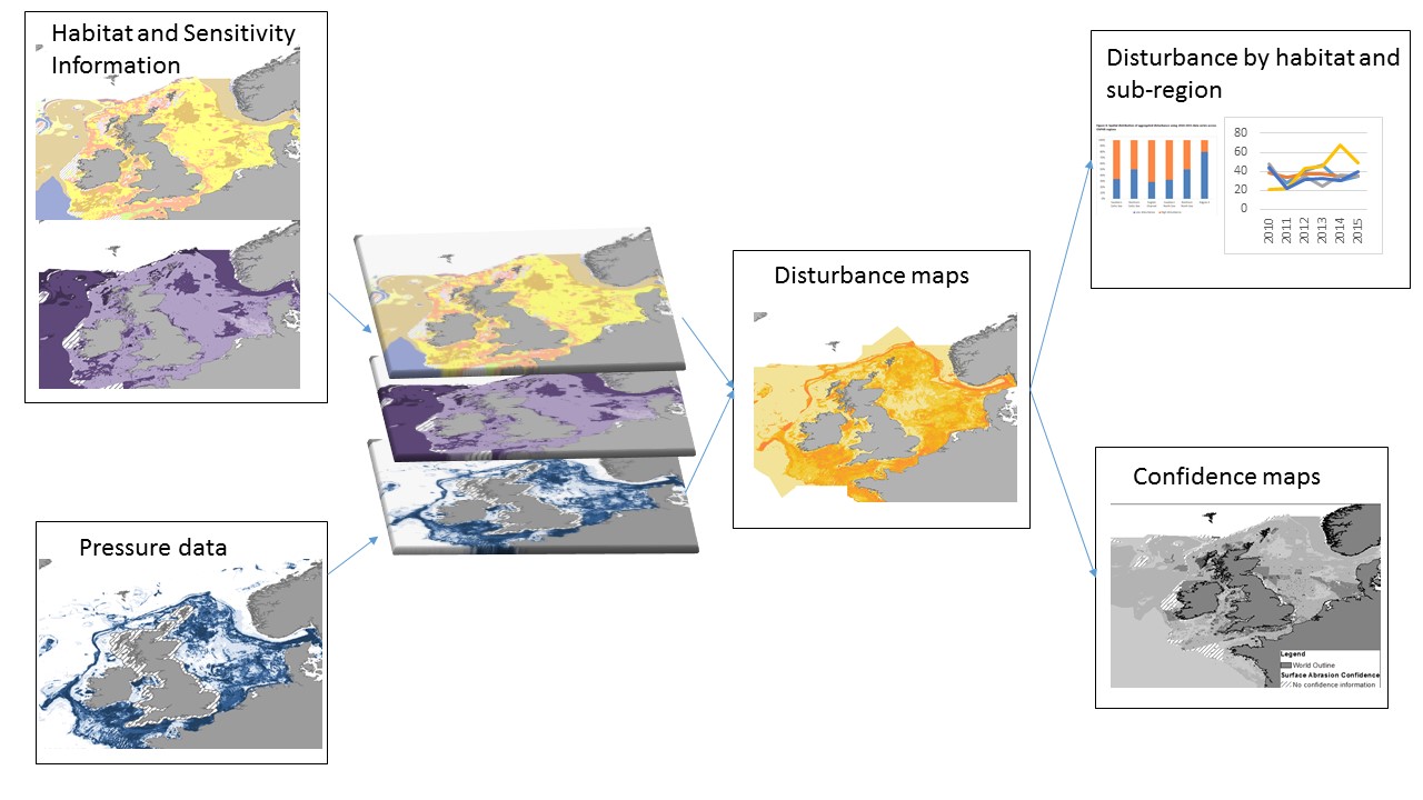
Figure a: Interlinkage between data inputs, processes and outputs for the physical damage indicator
The analysis has four components:
- A composite habitat map showing the extent and distribution of habitats (based on observational and modelled data), including the mapped extent of any relevant features (e.g. records and distribution of particular species and biotopes such as the European Nature Information System (EUNIS) Level 5 habitats or other biological characteristics). For this assessment a biotope is defined as the combination of an abiotic habitat and its associated community of species (Connor et al., 2004). All habitat data were combined at EUNIS level 3.
- Tables relating benthic habitat type to habitat sensitivity scores based on their resistance and resilience (i.e. recoverability) (Tillin et al., 2010; BioConsult, 2013; Tillin and Tyler-Walters, 2014). Sensitivity is assessed at species, biotope and EUNIS Level 3, depending on what habitat mapping information is available within each grid cell (c-square).
- Distribution and intensity of pressures causing physical damage. This analysis focused on surface and sub-surface abrasion caused by bottom trawling (for fishing from vessels >12 m only) within 0.05° grid cells (c-squares) (JNCC, 2011; ICES, 2015; Church et al., 2016).
- Distribution of levels of disturbance per habitat type per year. Calculation of disturbance is based on the intensity and duration of pressures and habitat sensitivity per pressure type. The pressures of abrasion (non-fisheries), siltation and selective extraction are not currently included in the assessment, but will be incorporated in future developments of the Indicator.
Data concerning the four components are combined using a step-wise approach to calculate the total area of different levels of disturbance, and a combination of those, across the region, per habitat type. The results are used to calculate variability in fishing intensity and trends in disturbance per year and for a six-year period.
The spatial assessment of this indicator is presented at EUNIS level 3, and has been prepared by combining the sensitivity and pressure data from habitats, biotopes and species within the EUNIS Level 3 habitat polygons. For this assessment the OSPAR regions have been sub-divided following biogeographic boundaries (OSPAR, 2016) into: Southern North Sea and Northern North Sea Southern Celtic Sea and Northern Celtic Sea English Channel and Bay of Biscay / Iberian Coast. For The Wider Atlantic, only a partial assessment has been possible owing to insufficient habitat and sensitivity data for the deep seafloor areas.
The methodology is based on a series of analytical steps that combine the distribution and intensity of physical damage pressures with the distribution and range of habitats and their sensitivities.
Step 1: Establishing Habitat Extent
An important component of this indicator is the production of a composite habitat map showing the extent and distribution of predominant and special habitats and their associated sensitivities. This map is produced using a combination of benthic survey data and modelled habitat maps (Figure b). As a basis for the assessment, a full coverage EUNIS Level 3 habitat map has been produced for the OSPAR Maritime Area, integrating maps from surveys and broad-scale models. The new EUNIS classification has not been used because it is still under development therefore version 2007-11 is used in this assessment.
The EUNIS habitats are mapped at different levels of detail, from Level 3 physical habitats to Level 6 biological communities and then aggregated to EUNIS Level 3 where more detail is provided. The majority of the habitat maps were obtained from the European Marine Observation and Data Network (EMODnet) Seafloor Habitats portal, including the broad-scale physical habitat map, EUSeaMap (EMODnet, 2010, 2016), and more detailed habitat maps created from survey data available through EMODnet, or as part of OSPAR habitat data calls. The information on the coverage and type of data were taken into account for the calculation of confidence maps (Step 6). The specification for a habitat map for the assessment of the Extent of Physical Damage indicator included the following conditions:
- To contain information on the relevant EUNIS habitat/biotope type at any level between Levels 3 and 6;
- To refer data on biotopes to Level 3 of the EUNIS habitat classification system;
- To use the broad-scale modelled map, EUSeaMap at EUNIS Level 3 when higher resolution maps from surveys are not available;
- To use the best available evidence on habitat data;
- To cover the greatest possible area of the OSPAR Maritime Area; and
- To contain no overlaps.
Mapping rules were established in order to decide objectively which of the overlapping datasets would be the sole occupant in the overlapping area. Where a EUNIS habitat map developed from survey data overlapped with a broad-scale predictive habitat map, a threshold confidence score of 58% was used as a simple rule for deciding whether to favour the habitat map from survey data. This threshold was based on the MESH protocol (Mapping European Seabed Habitats) (EMODnet, 2010). Within the MESH scoring system, for any map to have a score greater than 58%, the survey techniques must have used a combination of remote sensing and ground-truthing to derive the habitat types, hence physical and biological elements are included for its production. Therefore, 58% was deemed to be the lower threshold at which an overlapping survey map is considered to be of higher quality than the broad-scale predictive map. Pre-processing conditions and rules for the combining of data are available in the CEMP Guidelines (OSPAR, in prep).
Step 2: Assessing Habitat Sensitivity
The sensitivity of benthic habitats is determined based on a combination of the resilience (recoverability) and resistance (tolerance) of key structural, functional and characterising species of the habitat in relation to a defined intensity of each pressure (Tillin et al., 2010; BioConsult, 2013; Tillin and Tyler-Walters, 2014). Due to data limitations, the sensitivity scores are defined using a categorical scoring approach (Tillin et al., 2010). Sensitivity assessments for ecological groups have also been undertaken using Bray-Curtis cluster similarity analysis and Multidimensional Scaling, where resistance and resilience scores are assigned to groups of species with similar biological traits (e.g. burrowers) (Tillin and Tyler Walters, 2014).
The sensitivity map is created with three stages, using best available evidence where present (Figure e and Figure f):
- Stage one. Species records from survey data, that match a list of species assigned to a specific ecological group, are mapped using their maximum sensitivity value (based on the combination of resilience and resistance). Data are plotted as the intersection between the habitat polygon and a 0.05° grid.
- Stage two. If there is a high enough density of species recorded and agreement between the species and the underlying habitat they are within, then the sensitivity from the same species records used in stage one are used to assign a modal sensitivity to the surrounding habitat polygon. For example, if data coverage is sufficient, and the substrate and habitat type in the surrounding polygons are the same, then the same sensitivities are applied to these areas.
- Stage three. In order to act as a background map and to fill in areas not covered by the data collected from the first two stages, the habitat map outlined in Step 1 is used to assign EUNIS Level 3 benthic habitat sensitivities to the whole area. The sensitivities used in this step are often a range (from very low sensitivity to very high), in which case the maximum sensitivity is selected.
The maps are then combined geographically to show the highest confidence information across all regions.
Step 3: Assessing the Extent and Distribution of Physical Damage Pressures
For annual assessments the first task is to determine the relevant human activities causing physical pressures and their spatial and temporal extent. Bottom trawling is known to be affecting a large area of the seafloor (Dinmore et al., 2003; Eastwood et al., 2007; Foden et al., 2010, 2011; JNCC, 2011; Jennings et al., 2012) so the assessment method currently focuses on the corresponding pressures: surface abrasion (damage to seafloor surface features) and subsurface abrasion (penetration and / or disturbance of the substrate below the surface of the seafloor). Aggregated Vessel Monitoring System (VMS) fishing data are used to calculate the ‘swept area’ of a specific group of fishing gears (at the level of metier if this is available). Metier is a group of fishing operations targeting a similar (assemblage of) species, using similar gear, during the same period of the year and / or within the same area and which are characterised by a similar exploitation pattern.
The swept area is calculated using the parts of the fishing gear in contact with the seabed and is calculated on the width of fishing gear (in metres) multiplied by the average vessel speed (in knots) and the time fished. This calculation is undertaken on a cell-by-cell (grids or c-squares) basis per gear and per year, using data covering the six-year period 2010–2015 (see ICES Working Group Spatial Fisheries Data and CEMP Guidelines for Extent of Physical Damage to Predominant and Special Habitats (OSPAR, in prep) for the detailed method). Only the part of gear in contact with the seafloor is used for the analysis, and as a result all the gears have been classified according to type and/or metier group (Eigaard et al., 2015; Church et al., 2016). The swept area ratio (proportion of cell area swept per year; SAR) is then calculated by dividing the swept area by the grid cell area. The trawling effort is classified with an intensity scale ranging from ‘none’ to ‘very high’ (cell area swept more than 300% or three times per year). Separate Geographical Information System (GIS) layers are produced for surface abrasion and sub-surface abrasion. See Figure 1, Figure c, Figure d.
Assessments across a cycle (six years). To differentiate between cells with low and high SAR variability an analysis of variance is undertaken using the surface and sub-surface yearly results. This analysis allows the distinction between areas where fishing intensity seems to be consistent or at similar levels across years, and areas where fishing intensity levels fluctuates. A grid cell was considered to be ‘variable’ when the variance analysis showed a change in three or more categories of the classified SAR across all years.
In order to produce a layer showing the aggregated surface and sub-surface pressures that takes into account the variations in fishing pressures across years, a generic rule was used:
- For cells with low variability (i.e. under similar fishing pressure year on year) the mean of SAR across all years is calculated
- For cells with high variability (i.e. fishing pressure variable) the highest SAR value across all years is selected to define the pressure category because it represent the maximum level of exposure within the cycle. In this case, the maximum values, instead of mean were chosen to capture the highest level of damage caused by the initial impact of the first pass, which is regarded to be most damaging for benthic habitats. Due to the short timescales, it is not anticipated that the habitats will have recovered at the end of the assessment period, hence the approach captures the maximum level of damage per grid across all years. A change of three categories or more on the fishing pressure in the same grid across years is considered to be highly variable.
Step 4: Combining Pressure Intensity and Habitat Sensitivity
The degree of disturbance of a habitat is a prediction based on the spatial and temporal overlap of its sensitivity and exposure to a specific pressure. Sensitivity and pressure are combined via a matrix, producing ten categories of disturbance (0–9, where 0 is no disturbance and 9 is the maximum disturbance possible). The matrix was created from the result of previous studies that looked at the impacts of pressures on sensitive species and habitats when applied at different levels of intensities (Schroeder et al., 2008; BioConsult, 2013). The matrix is used to calculate the disturbance for each surface and sub-surface abrasion per year. These disturbance maps are then combined by selecting, for each of the cells, the highest disturbance category from the two pressure layers (Figure 2, Figure g, Figure m).
At present, other activities that could cause physical damage pressures, are not included. It is anticipated that due to the different nature of the pressures ‘selective extraction’, ‘abrasion’ and ‘changes in siltation’, separate disturbance matrices or algorithms will be required which will take into account the spatial distribution of pressures and the temporal effects. This information is not currently available and will be included in the next assessment cycle for an overall calculation of disturbance caused by physical damage.
Step 5: Disturbance Aggregation Method and Trend Analysis
Disturbance values across years are combined using the aggregated fishing pressure spatial layers, developed in Step 3. Results are used to calculate trend between years in those grid cells or c-squares identified as variable. This allows the variation of disturbance across years per habitat type to be assessed. The trend analyses are simple plots over the six-year period, rather than a linear regression, which was not possible due to the small number of years assessed (Figure l).
The disturbance categories were aggregated into two groups: disturbance categories 0–4 (representing lower levels of disturbance) and disturbance categories 5–9 (representing higher levels of disturbance). This scale is the result of a combination of the temporal variation of fishing activity and the range of sensitivity values.
Step 6: Confidence assessments
In order to spatially represent confidence in the data, a numeric method of calculating confidence was adapted from an internal OSPAR method. The method multiplies relative measures of confidence on a scale of 0–1, where there is a difference in confidence between categories or classes used in a data layer.
A numerical score (0.33, 0.66 or 1) was manually assigned by the assessor to each of the different attributes used to create the sensitivity layer. A high confidence score was given a numeric value of 1, medium 0.66 and low 0.33. The different methods used to create the sensitivity layer were taken in turn and a numeric confidence score was assigned to each of the attributes: confidence based on underlying data (Figure q); confidence within data source (such as MESH confidence for habitats); and confidence in the sensitivity of the habitat to a pressure.Résultats
Cette évaluation préliminaire de l’indicateur révèle la répartition et l’intensité des pressions exercées par les activités de pêche de fond et les perturbations correspondantes du sol marin à l’échelle régionale OSPAR. L’approche conjugue des approches semi-quantitatives et des approches catégoriques appliquées au rapport pression / impact entre les habitats et la pêche. Il n’est pas possible d’utiliser une méthode complètement quantitative à ce stade car elle limiterait les résultats à des sites à petite échelle ou lorsque des séries de données à long terme sont disponibles.
La figure 1 montre la répartition de l’abrasion de surface causée par les navires d’une longueur supérieure à 12 m utilisant des engins de pêche de fond, agrégée pour les années de 2010 à 2015. Les zones comportant une abrasion de surface de faible niveau, voire aucune, causée par la pêche (par exemple nord-ouest de l’Irlande du Nord) se distinguent de celles subissant des niveaux plus importants d’activité (par exemple, la Manche, le Skagerrak et le Kattegat). Dans l’ensemble, 74% des cellules de la grille évaluées ont subi des pressions régulières d’année en année, les 26% restantes révélant une variabilité élevée (on considère qu’une modification d’au moins trois catégories des pressions exercées par la pêche dans la même grille au fil des ans indique une variabilité élevée). Il s’agit d’un facteur important pour une analyse ultérieure des perturbations car la manière dont les pressions varient dans le temps va affecter la capacité de récupération des habitats. Ceci signifie que les zones à haute variabilité seront à des stades différents de récupération et d’impact.
La figure 2 montre les valeurs agrégées des perturbations à la surface du sol marin et dans le sous-sol pendant la période de 2010 à 2015. Le niveau le plus élevé des perturbations se trouve dans les mers Celtiques méridionales, 76% de cette zone étant soumise à des perturbations élevées (catégories 5–9). Les perturbations dans la Manche et la mer du Nord méridionale sont légèrement inférieures, 72% et 68% respectivement. Au sein de chaque zone d’évaluation, il y a des cellules de la grille qui ne révèlent aucune perturbation ou des perturbations faibles (catégories 0–4), telles que certaines zones de la mer du Nord septentrionale.
Il s’agit de la première évaluation, à l’échelle d’OSPAR, des perturbations physiques causées aux habitats benthiques. Ainsi, la méthodologie utilisée inspire une confiance faible / modérée. La disponibilité des données inspire une confiance faible (mais de modérée à élevée dans les zones bien surveillées).
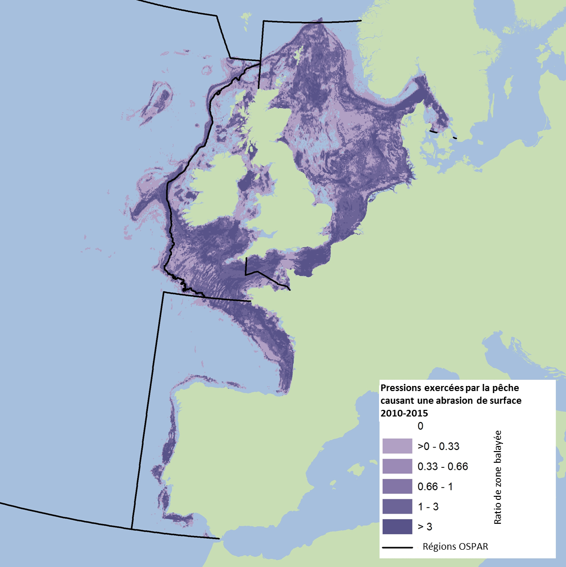
Figure 1: Pressions agrégées causant une abrasion de surface, utilisant les séries de données de 2010 à 2015. L’unité de pression est le ratio de zone balayée (proportion de la cellule de la grille balayée par engin de pêche)
La zone hachurée autour du Royaume-Uni indique les zones où les activités de pêche côtière à partir de navires d’une longueur <12 m sont supérieures à celles à partir de navires d’une longueur >12 m.
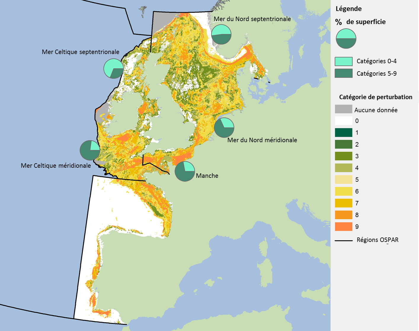
Figure 2: Répartition spatiale des perturbations agrégées utilisant les séries de données de 2010 à 2015 dans les sous-régions OSPAR
Catégories de perturbations allant de 0 à 9, 0 correspondant à aucune perturbation et 9 aux perturbations les plus importantes. Les plots indiquent le pourcentage de la superficie des sous-régions OSPAR dans les catégories de perturbation de 0 à 4 (aucune ou peu de perturbation) et de 5 à 9 (perturbations importantes) au cours du cycle de notification (2010–2015). Le pourcentage correspondant au golfe de Gascogne et à la côte ibérique n’a pas été inclus car les données étaient incomplètes.
Composite Habitat map
An overview of the method used to run the indicator assessment as provided in this assessment sheet can be seen in Figure a. The first step in this assessment produces a composite map of habitat data, using mainly EMODnet (interim version 2016) layers along with survey maps (Figure b, Table a) and provides a spatial overview of the extent and distribution of predominant habitat types across the OSPAR Maritime Area. This spatial model integrates most of the existing survey biotope data and modelled maps at different European Nature Information System (EUNIS) levels combined for a final aggregation at EUNIS Level 3.
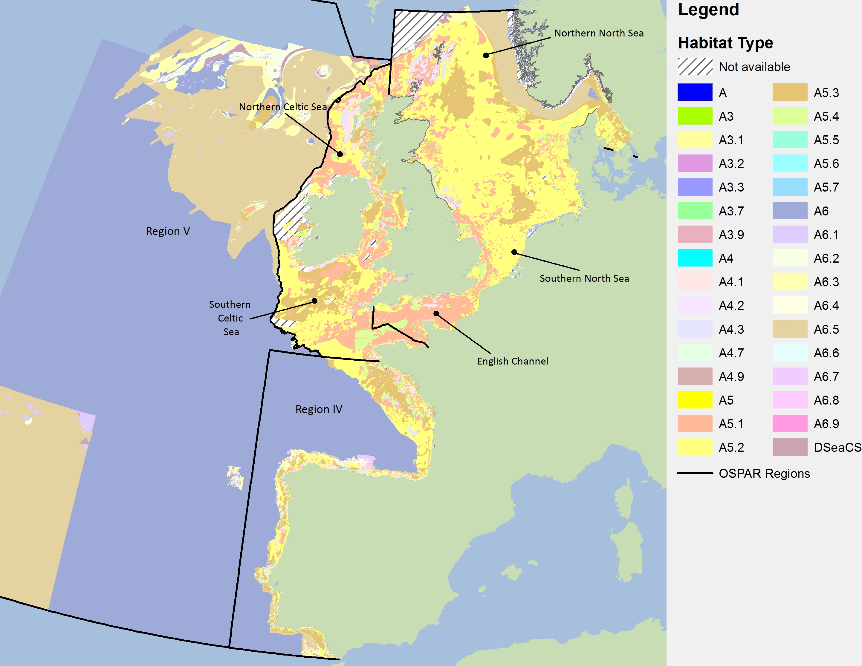
Figure b: OSPAR-scale full-coverage EUNIS Level 3 benthic habitat map, integrating maps from surveys and broad-scale models
OSPAR Region/ Sub-Region Codes: NNS= Northern North Sea, SNS= Southern North Sea, CH= English Channel, NCS= Northern Celtic Sea, SCS= Southern Celtic Sea, I= Arctic Waters, IV= Bay of Biscay and Iberian Coast, V= Wider Atlantic. Full legend explanation for benthic habitat codes can be found in table a.
| EUNIS Code | Habitat Description |
|---|---|
| A3.1 | High energy infra littoral rock |
| A3.2 | Moderate energy infra littoral rock |
| A3.3 | Low energy infra littoral rock |
| A3.7 | Features of infra littoral rock |
| A4.1 | High energy circalittoral rock |
| A4.2 | Moderate energy circalittoral rock |
| A4.3 | Low energy circalittoral rock |
| A4.7 | Features of circalittoral rock |
| A5.1 | Subtidal coarse sediment |
| A5.2 | Subtidal sand |
| A5.3 | Subtidal mud |
| A5.4 | Subtidal mixed sediments |
| A5.5 | Subtidal macrophyte-dominated sediment |
| A5.6 | Subtidal biogenic reefs |
| A5.7 | Features of sublittoral sediments |
| A6.1 | Deep-sea rock and artificial hard substrata |
| A6.2 | Deep-sea mixed substrata |
| A6.3 | Deep-sea sand |
| A6.4 | Deep-sea muddy sand |
| A6.5 | Deep-sea mud |
| A6.6 | Deep-sea biotherms |
| A6.8 | Raised features of the deep-sea bed |
All regions have a large variety of habitats with the most widespread being soft sediments. There are some habitat layers missing from the map for the west coast of Ireland due to the substrate layers not being available in time for the assessments. The availability of biotope (EUNIS habitat Level 5 and below) survey maps will increase the quality of the composite map being produced for this Indicator in the future.
Abrasion Pressures and Disturbance
The extent of the sub-surface abrasion pressure, caused by parts of fishing gears that penetrate deep into sediment, is generally less than the extent of surface abrasion pressure (Figure c). The highest intensities of sub-surface abrasion are along the Dutch, German and Belgian coastlines, the Skagerrak/Kattegat areas, and some areas along the English Channel and to the south of Brittany (France). The data from the sub-surface abrasion contribute to the overall pressure.
It should be noted that the surface and sub-surface pressures maps (Figure 1 and Figure c) do not capture all bottom fishing activity. For example, Spanish fleet data are missing from the SAR calculations. It is expected that some data are missing or potentially misallocated due to different approaches for extracting data from national databases. A gap also exists around the activities of smaller vessels (<12 m) fishing using bottom contacting gear, mostly in coastal waters that are not equipped with a Vessel Monitoring System (VMS) transmitter. This is an important issue for countries such as the UK, where small vessels represent the largest proportion of the fleet operating within inshore waters (less than 12 nautical miles of the coast). These issues will be addressed as the Indicator is further refined.
For the analysis at OSPAR level only aggregated VMS and logbook data per grid cell are available (VMS ping data points are not available because of confidentiality issues), and grouped by gear type (e.g. otter trawl). As a result, there is likely to be an over-estimation of the results for both surface and sub-surface abrasion in some areas, as each grid cell has a unique SAR value that assumes a homogenous distribution of fishing. However, this can be partially addressed if the existing information from gear types at level 6 (metiers) are made available for this analysis.
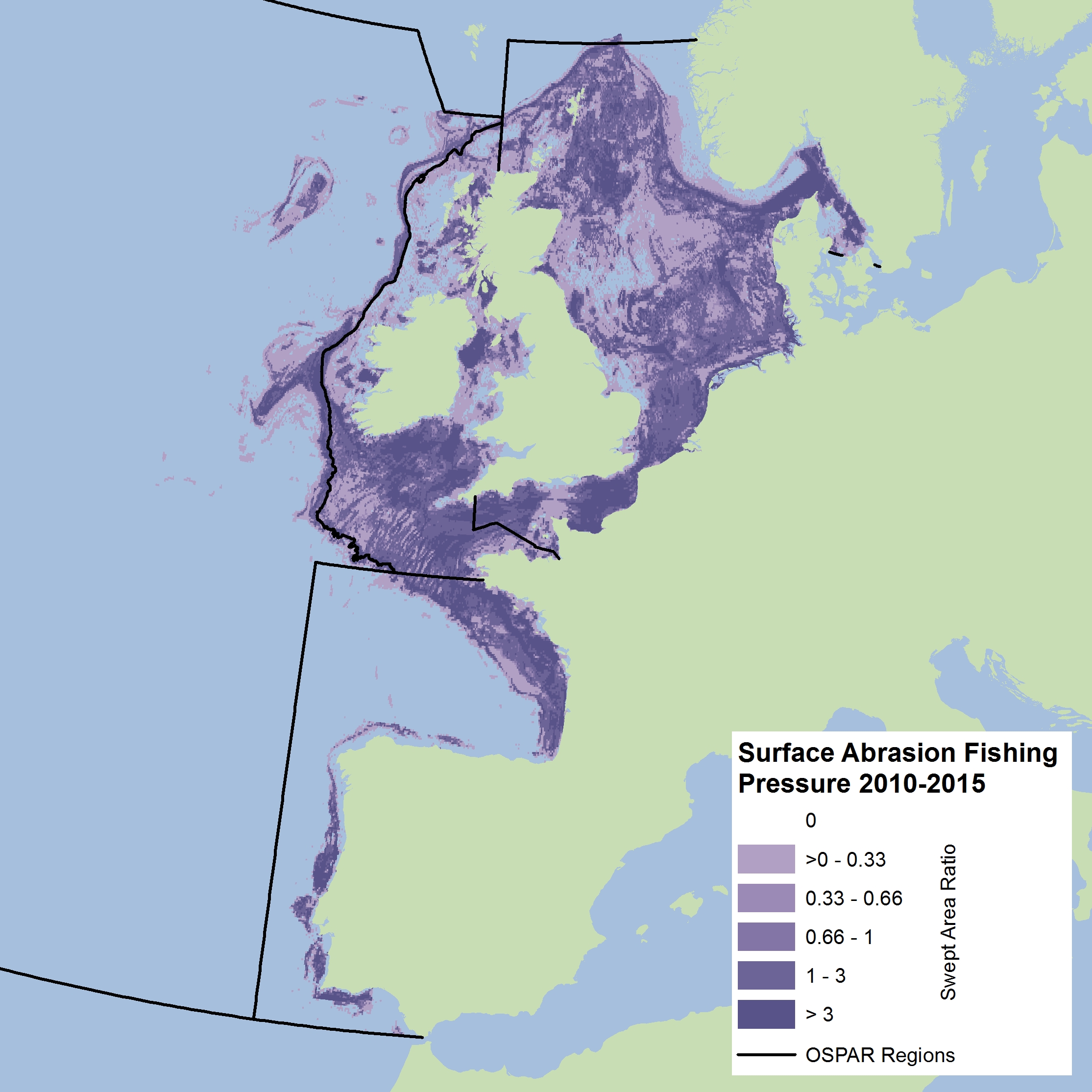
Figure c: Aggregated sub-surface abrasion pressure using the 2010–2015 data series
Pressure unit is swept area ratio (the proportion of grid cell swept by fishing gear). The hatched area around the UK shows the areas where inshore fisheries activity from vessels <12 m in length is higher than those >12 m in length.
Pressure Variability Across Years
In order to aggregate the pressure maps for the assessment period (2010–2015) and to detect trends in pressure intensity, cells with consistent pressure were distinguished from those with high variability (Figure d, Table b). The calculations to determine variability were undertaken using an analysis of variance (trend analyses were not statistically viable due to the limited number of years available). An area with especially high variability is the Northern North Sea, whereas in other assessment areas, most of the area experiences consistent levels of pressure intensity. For example, some of the grid cells in the eastern parts of the English Channel are under the same level of pressures across all years, all have a SAR of more than 3. However, in some areas off the western coast of Scotland some grid cells showed changes in the pressure categories from 3.6 in 2010 to no fishing in 2011, 2014 and 2015.
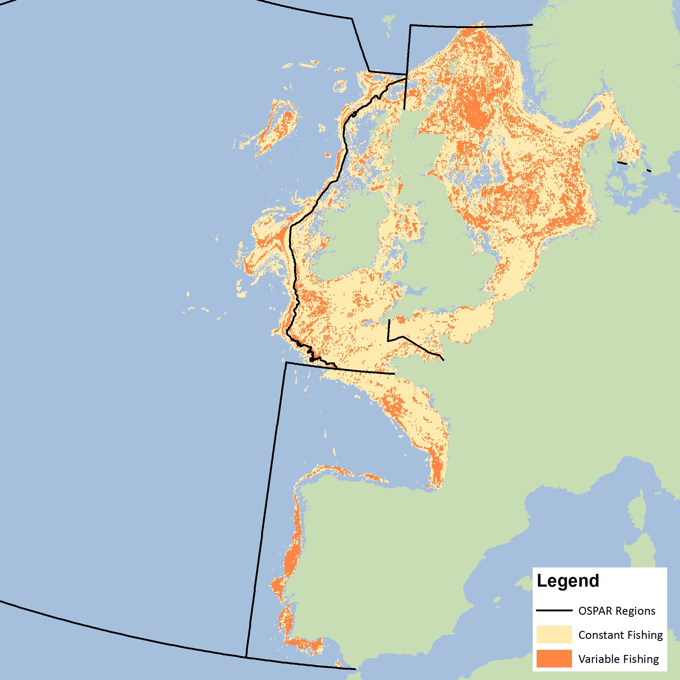
Figure d: Spatial distribution of variable and consistent fishing using the 2010–2015 data series
Variable fishing is said to occur if a grid cell has a change in three or more pressure categories.
| Fishing variability | Number of grid cells (c-squares) | Area (km²) | Percentage of grids (c-squares) |
|---|---|---|---|
| Highly Variable Fishing | 23,479 | 321,800 | 26% |
| Constant Fishing | 66,302 | 894,500 | 74% |
Habitat Sensitivity Results
The distribution of habitat sensitivity to surface and subsurface abrasion has been calculated using the method outlined in the previous section; it should be noted that, in calculating sensitivity both resistance and resilience are considered. The extent to which a habitat is disturbed is affected by the ability of the habitats to withstand the impacts (resistance) and to recover after subsequent events (resilience) (Tillin et al., 2010). Therefore, resilience is a key element to assess the temporal effects of pressures. Regional variation in the sensitivity of habitats to surface and sub-surface abrasion are shown in Figure e and Figure f. There are some differences between the surface and sub-surface sensitivities, but overall medium-range sensitivity (score of 3) is the most common. Habitats that have been assigned the highest level of sensitivity to abrasion are rocky, biogenic reefs and deep-sea habitats (score of 5).
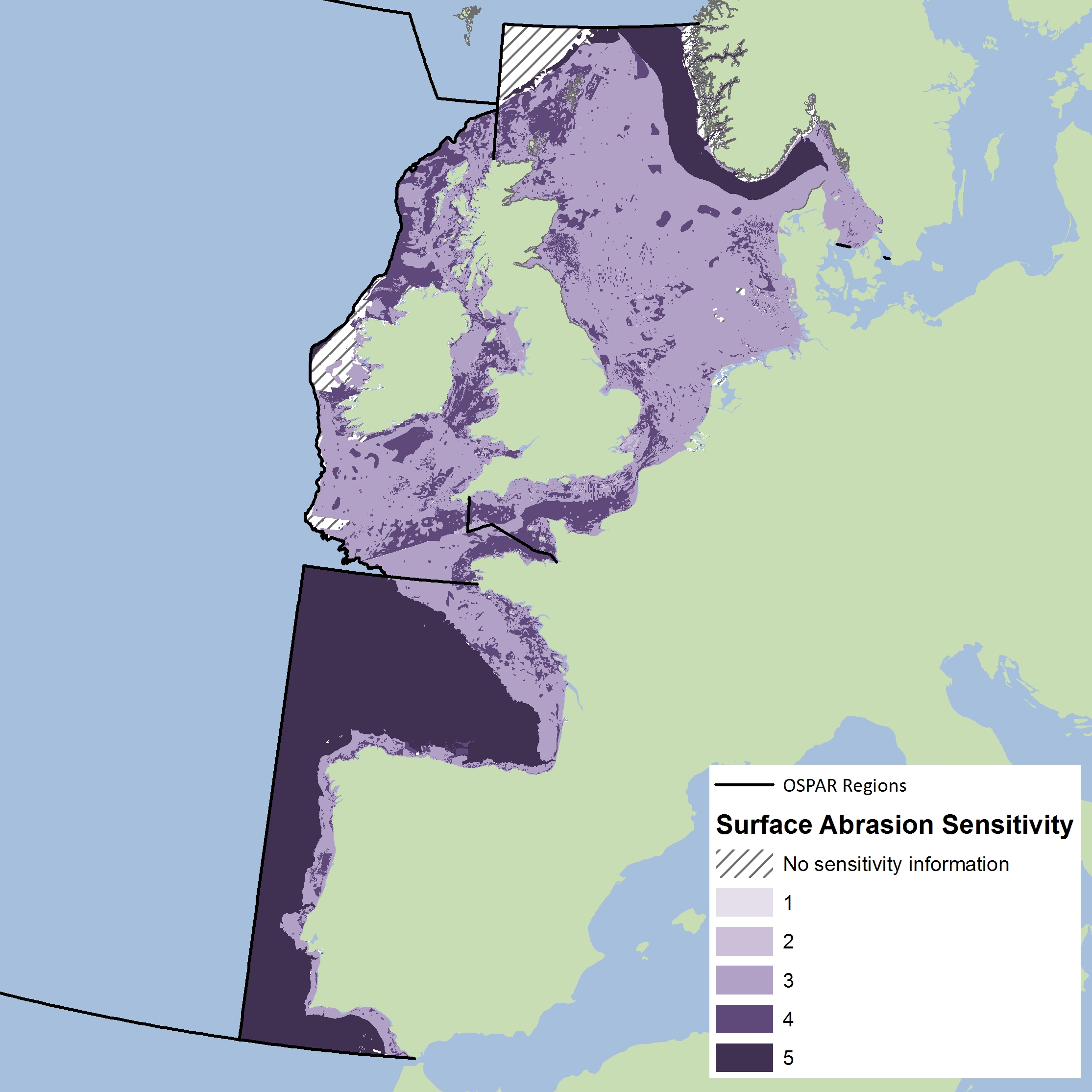
Figure e: Extent and distribution of habitat and benthic species sensitivities (based on resilience and resistance) to surface abrasion combined within EUNIS Level 3 benthic habitat types
Sensitivity is expressed in categories from 1–5, where 1 is the least sensitive and 5 is the most sensitive.
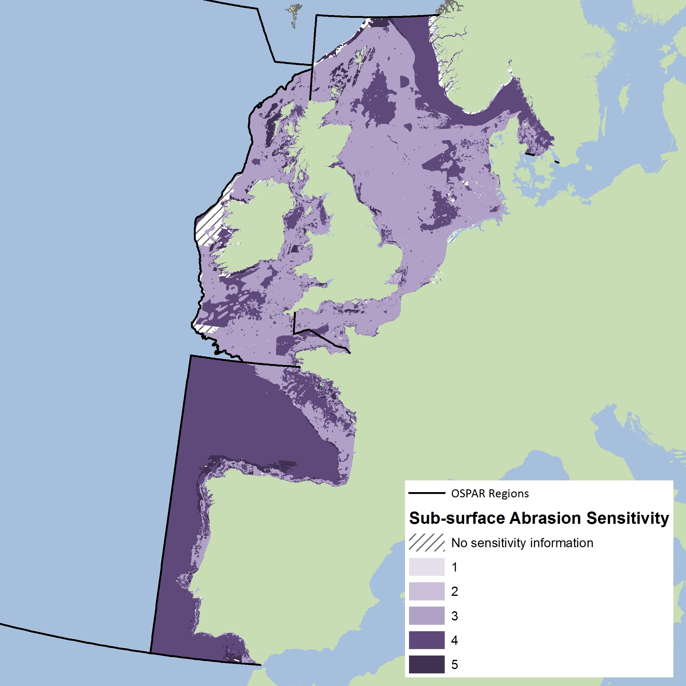
Figure f: Extent and distribution of habitat and benthic species sensitivities (based on resilience and resistance) to sub-surface abrasion combined within EUNIS Level 3 benthic habitat types
Sensitivity is expressed in categories from 1–5, where 1 is the least sensitive and 5 is the most sensitive.
Assessment by Region
The spatial distribution of disturbance aggregated across the six-year assessment period (2010–2015) has been split by assessment area, in order to present the distribution within the regions more clearly (Figures g-k). The results should be used in combination with habitat distribution in Figure b. An overview of the area of disturbance is presented in Table c.
Southern and Northern Celtic Seas (Celtic Seas)
The majority of the Southern Celtic Sea (Figure g) grid cells have some level of disturbance value. The highest disturbance occurs mostly on coarse sediments followed by mud habitats, whereas in the Northern Celtic Sea (Figure h), disturbance distribution is patchier, with the highest levels mostly occurring on areas of sublittoral mud off the east coast of Northern Ireland and the west coast of Scotland, and deep-sea mud from the west of Ireland. Both assessment areas are showing temporal variations (Figure l).
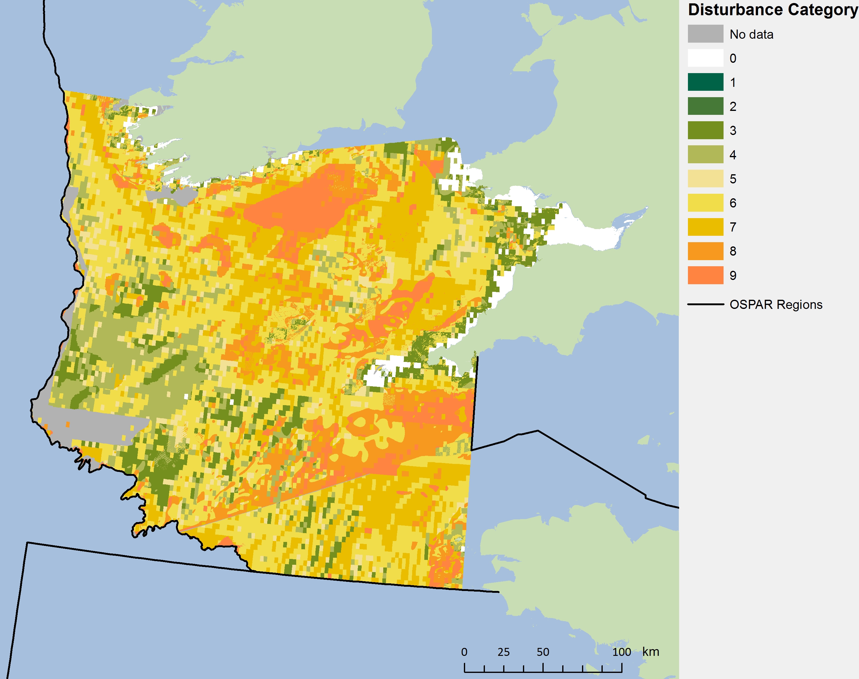
Figure g: Spatial distribution of aggregated disturbance using the 2010–2015 data series across OSPAR sub-region Southern Celtic Sea
Disturbance categories 0–9, with 0= no disturbance and 9= highest disturbance.
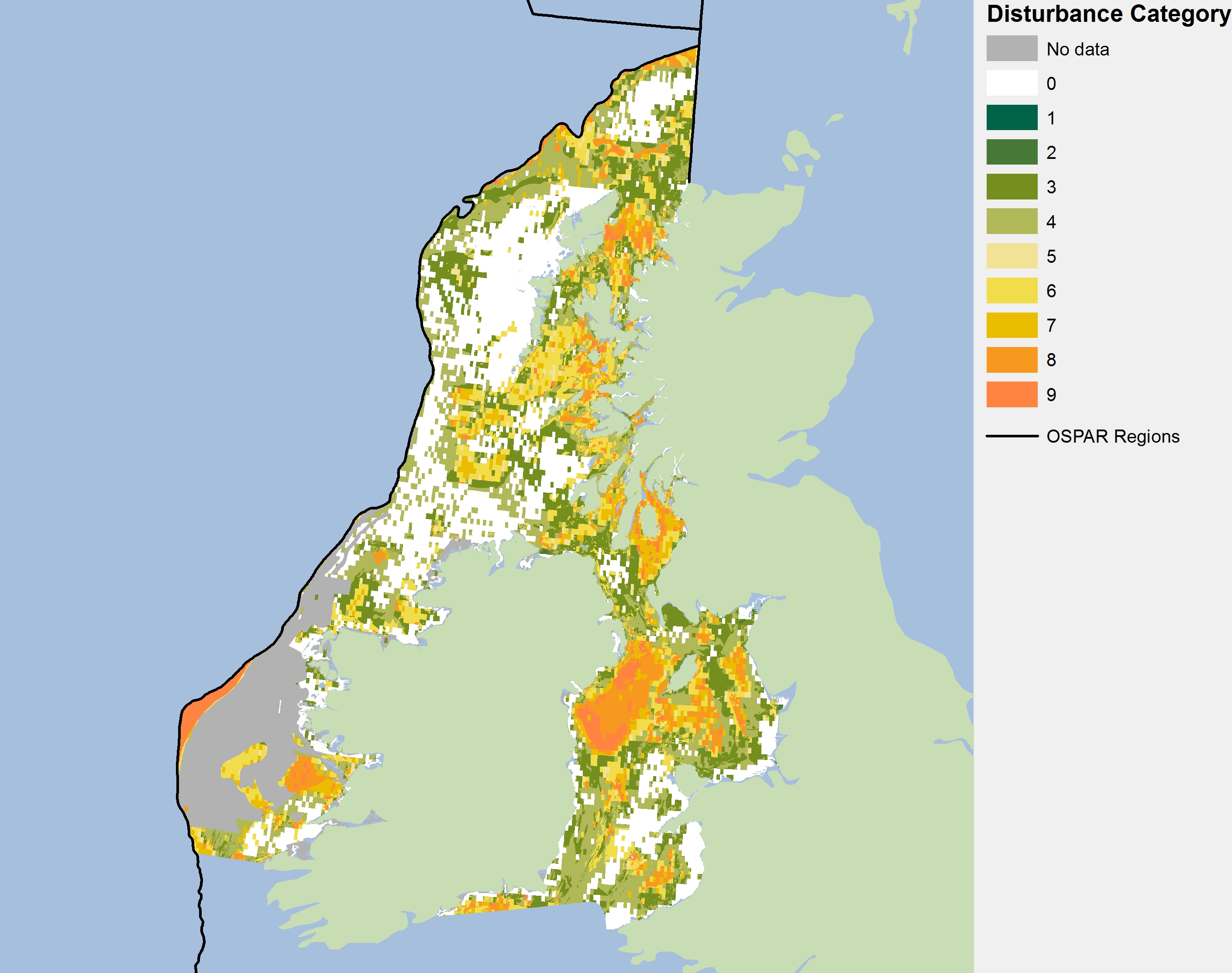
Figure h: Spatial distribution of aggregated disturbance using the 2010–2015 data series across OSPAR sub-region Northern Celtic Sea
Disturbance categories 0–9, with 0= no disturbance and 9= highest disturbance.
Southern and Northern North Sea (Greater North Sea)
In the Northern North Sea (Figure i), some areas show no or very low levels of disturbance, with the highest proportions of disturbance on sand and mud habitats, especially those along the northerly shelf edge of Great Britain and the Norwegian Trench to the Skagerrak. It should be noted that in most cases the pattern of disturbance follows the distribution of predominant habitats and depth contours along the shelf. There is high variability in disturbance (Figure j) across the entire Southern North Sea assessment area, with the highest values to the south, centre and north-east.
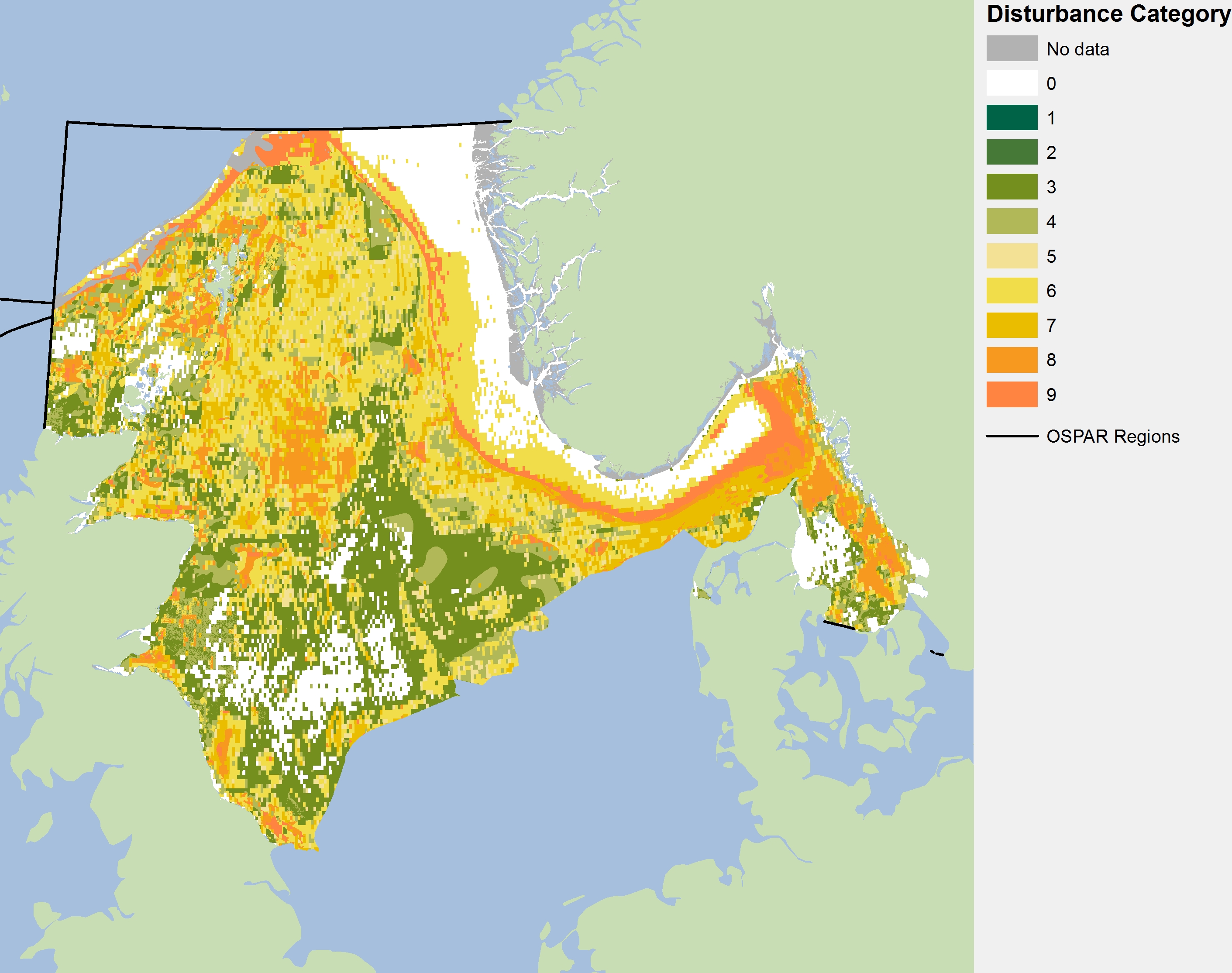
Figure i: Spatial distribution of aggregated disturbance using the 2010–2015 data series across OSPAR sub-region Northern North Sea
Disturbance categories 0–9, with 0= no disturbance and 9= highest disturbance.
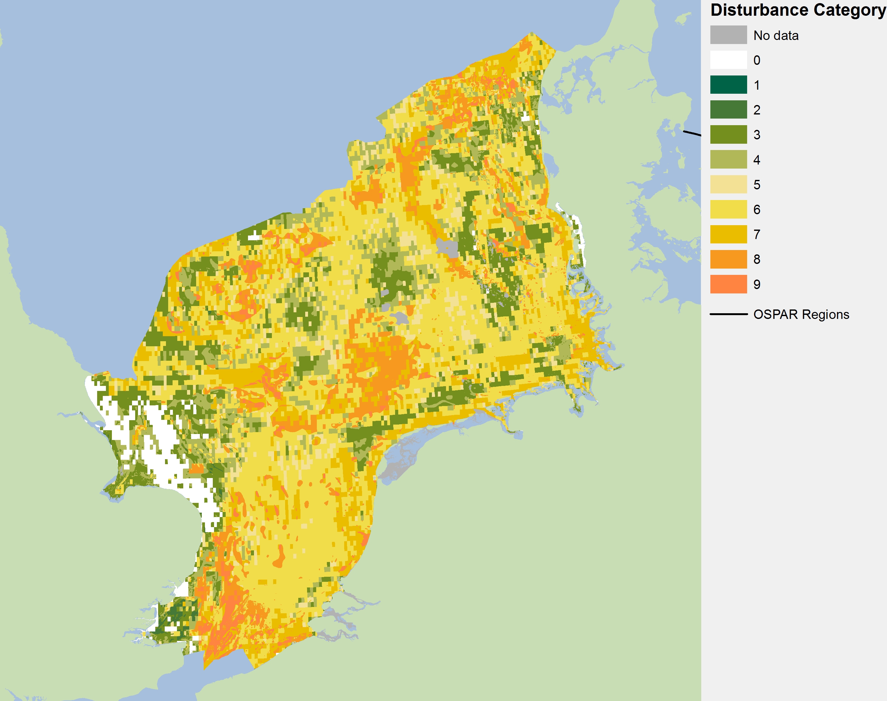
Figure j: Spatial distribution of aggregated disturbance using the 2010–2015 data series across OSPAR sub-region Southern North Sea
Disturbance categories 0–9, with 0= no disturbance and 9= highest disturbance.
English Channel (Greater North Sea)
The English Channel shows the highest proportion of disturbance on coarse sediment off the west coast of the Cotentin Peninsula in Normandy and the south-west of England, with very low disturbance north of the Cotentin Peninsula and north of Brittany (Figure k), although trend analysis shows a slight decrease in disturbance between 2012 and 2015 in this assessment area (Figure l).
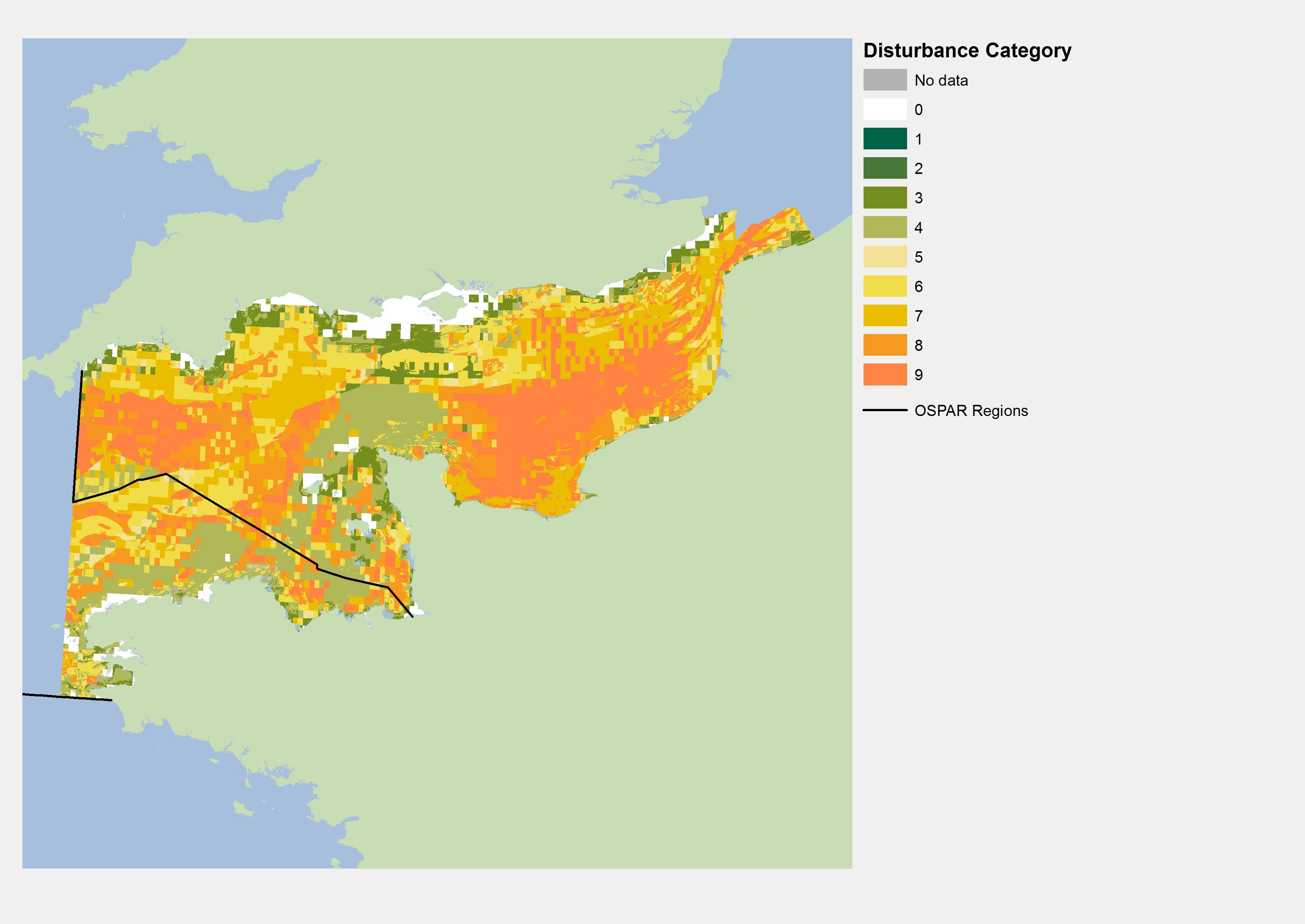
Figure k: Spatial distribution of aggregated disturbance using the 2010–2015 data series across OSPAR sub-region English Channel
Disturbance categories 0–9, with 0= no disturbance and 9= highest disturbance
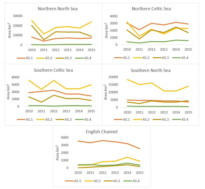
Figure l: Trend analyses for a selection of habitats (A5.1- sublittoral coarse sediment, A5.2- sublittoral sand, A5.3- sublittoral mud and A5.4- sublittoral mixed sediments) per sub region for area with disturbance in categories 5–9
Only cells with high variability in fishing pressure are shown
| Area (km²) | Percentage of area | |
|---|---|---|
| Area in disturbance categories 1-9 | 912,353 | 86% |
| Area in disturbance categories 5-9 | 609,353 | 58% |
Bay of Biscay and Iberian Coast
The Bay of Biscay and Iberian coast region is not assessed due to the lack of complete data.
Assessment by Habitat Type
The level of disturbance within a habitat type varies, as demonstrated in Figure m, which shows the distribution of disturbance categories for sublittoral mud (A5.3). The variability is mainly driven by the differences in fishing pressure causing surface and subsurface abrasion within a habitat across the regions. For example, in the Celtic Seas, the distribution of fishing effort on sublittoral mud is constrained by the patchy and localised distribution of this habitat type; the Northern Celtic Sea has the highest level of disturbance categories (8 and 9), whereas in the Southern Celtic Sea most of this habitat type shows disturbance above category 4.
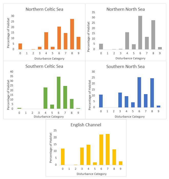
Figure m: Distribution of disturbance categories for the habitat A5.3, Subtidal mud for OSPAR sub-regions
Table d shows the percentages of habitat area with high levels of disturbance (categories 5–9) for all EUNIS Level 3 habitats per assessment area included in the assessment. Nearly all deep-sea habitats that are subject to fishing pressure in these areas are experiencing high disturbance, as the sensitivity of these habitats is determined as very high. The region showing the highest level of disturbance is the Southern Celtic Sea with more than 75% of the main soft sediments (sand, mud, coarse and mixed sediments) showing disturbance of categories 5 and above. Sublittoral sands have the highest percentage of disturbance in the Southern Celtic Seas, Southern North Sea and English Channel (above 70%). In contrast, infra-littoral habitats generally experience lower disturbance. Overall, the results for sublittoral soft sediments are highly variable across regions.
| Bay of Biscay and Iberian Coast | Northern Celtic Sea | Southern Celtic Sea | English Channel | Southern North Sea | Northern North Sea | |||||||
|---|---|---|---|---|---|---|---|---|---|---|---|---|
| Area (km²) | % | Area (km²) | % | Area (km²) | % | Area (km²) | % | Area (km²) | % | Area (km²) | % | |
| A3.1 | 31 | 3 | 67 | 4 | 3 | 1 | 103 | 11 | 0 | 0 | 46 | 8 |
| A3.2 | 19 | 5 | 42 | 14 | 1 | 3 | 65 | 33 | 0.01 | 4 | 27 | 6 |
| A3.3 | 1 | 3 | 32 | 21 | 1 | 11 | 6 | 16 | 0 | 0 | 5 | 4 |
| A3.9 | 0 | - | 0 | - | 0 | - | 142 | 61 | 0 | - | 0 | - |
| A4.1 | 3022 | 65 | 3153 | 30 | 1531 | 54 | 1938 | 75 | 20 | 40 | 1692 | 65 |
| A4.2 | 1714 | 49 | 2621 | 48 | 1445 | 74 | 716 | 84 | 53 | 20 | 5488 | 78 |
| A4.3 | 2248 | 40 | 591 | 16 | 285 | 68 | 1 | 33 | 0 | - | 3228 | 44 |
| A4.7 | 0 | - | 0 | - | 0 | - | 0 | - | 0 | - | 0 | - |
| A5.1 | 10773 | 69 | 8964 | 16 | 37633 | 80 | 39030 | 72 | 16183 | 56 | 17344 | 41 |
| A5.2 | 31537 | 61 | 11604 | 29 | 52121 | 75 | 7633 | 73 | 73083 | 72 | 83544 | 47 |
| A5.3 | 23680 | 63 | 15308 | 77 | 25434 | 76 | 754 | 61 | 19450 | 67 | 48270 | 78 |
| A5.4 | 6698 | 71 | 1730 | 23 | 6320 | 95 | 7382 | 76 | 3396 | 49 | 3002 | 36 |
| A5.5 | 3 | 13 | 6 | 4 | 0.3 | 1 | 1 | 3 | 0 | 0 | 3 | 10 |
| A5.6 | 0 | - | 0 | 0 | 2 | 11 | 21 | 77 | 37 | 8 | 10 | 17 |
| A6.1 | 427 | 15 | 0 | - | 0 | - | 0 | - | 0 | - | 215 | 48 |
| A6.2 | 287 | 46 | 3 | 84 | 19 | 88 | 0 | - | 0 | - | 1416 | 75 |
| A6.3 | 4270 | 36 | 92 | 100 | 55 | 100 | 0 | - | 0 | - | 5412 | 96 |
| A6.4 | 286 | 22 | 0 | - | 0 | - | 0 | - | 0 | - | 0 | - |
| A6.5 | 6840 | 47 | 1270 | 100 | 165 | 100 | 0 | - | 0 | - | 28100 | 47 |
| A6.6 | 3 | 1 | 0 | - | 0 | - | 0 | - | 0 | - | 0 | - |
An analysis of disturbance values across years for the most widespread habitat types (only grid cells with high fishing variability) shows temporal and regional variations (Figure l and n). Sublittoral sand and mud habitats in the Northern North Sea, Northern Celtic Sea and the Southern Celtic Sea are especially subject to high variations in fishing pressure. In 2011, a strong decrease in disturbance of sublittoral sand and mud occurred in these assessment areas, followed by an increase in 2012. A similar, but less pronounced trend for sublittoral sand is also visible in the Southern North Sea, whereas there are generally no large changes in levels of disturbance in this assessment area for other habitat types. In the English Channel there appears to be a decrease in fishing pressure on sublittoral coarse sediment, which is the habitat with by far the greatest coverage, but the disturbance of sublittoral sand has increased in this region.
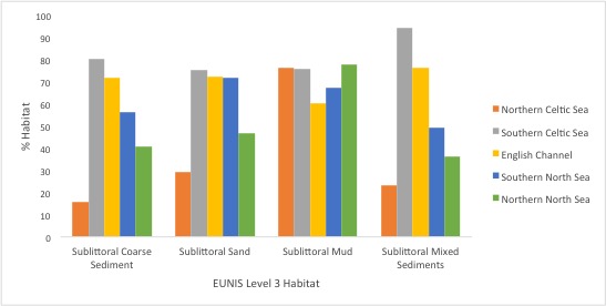
Figure n: Percentage of total area of each habitat in disturbance category 5–9 in each of the OSPAR sub-regions for coarse, sand, mud and mixed sediments
Assessment of OSPAR Threatened and / or Declining Habitats
Figure o shows the distribution of the different disturbance values for OSPAR Threatened and Declining habitats across all regions, while Figure p shows the habitat with the greatest disturbance is ‘seapen and burrowing megafauna communities’ with half of this habitat in the disturbance categories of 5 or above, followed by seamounts and Zostera beds. Distribution of the mostly small habitat areas is often unknown, and so confidence in these results is low.
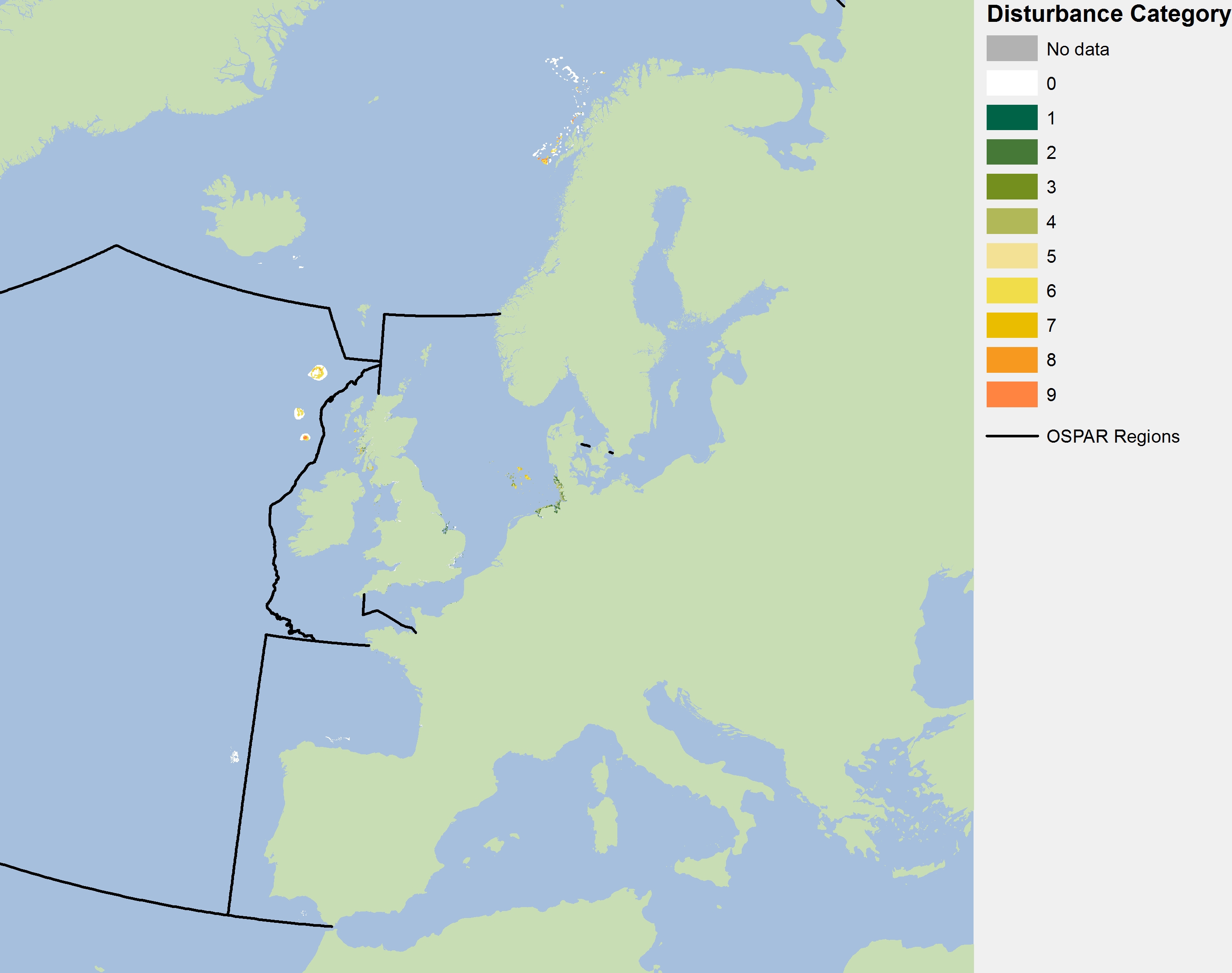
Figure o: Distribution of disturbance categories on OSPAR threatened and declining habitats using the aggregated fisheries time series for 2010–2015
Habitats shown: carbonate mounds, coral gardens, deep-sea sponge aggregations, Lophelia pertusa reefs, maerl beds, Modiolus modiolus beds, Ostrea edulis beds, seapen and burrowing megafauna, seamounts, and Zostera beds.
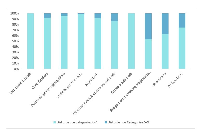
Figure p: Percentage area of OSPAR Threatened and Declining Habitats falling within disturbance categories 0–4 and 5–9 for the 2010–2015 time series
The availability of habitat data for these habitats is very patchy so the assessments were limited across the assessed areas. For example, some areas within the Celtic Seas, sublittoral mud (A5.3 habitat) could be classified as ‘seapen and burrowing megafauna communities’ but are not recorded as such in the OSPAR habitat database, and so the available habitat data only give a partial view of the real level of disturbance and overall physical damage on this special habitat type within and across the Celtic Seas assessment areas. There is an opportunity to improve the assessments of these habitats if additional information from benthic species collected during surveys can be added to increase the quality of the results. This will also help improve the evidence available on the distribution of sensitivity information across the regions.
Levels of Confidence
This is a first OSPAR-wide assessment of physical damage to benthic habitats. The method is based on Article 17 of the European Union Habitats Directive and vulnerability assessments of Marine Protected Areas. These have been used in several publications and for some European Union Member States in reporting on their implementation of the Habitats Directive. The method has been adapted for assessments of predominant habitats. There is recognition that the method needs further development and hence confidence for this assessment is rated as low/moderate.
A numeric method for calculating confidence has been developed (Figure q). At a regional scale the overall confidence in data availability for this assessment is low but there is high spatial variability in confidence scores. Higher confidence occurs around well-surveyed areas and much lower confidence where the assessment relies on modelled habitat maps.
The resulting disturbance values for benthic habitats must be viewed alongside the confidence map (Figure q). This map provides an indication of the type and source of habitat and sensitivity data underpinning the results. Confidence in the sensitivity scores, which are based on the level of data used and the quality of information available on the resistance and resilience of habitats and species to physical damage pressures (i.e. sensitivity scores derived from experimental or field survey studies have high confidence, whereas scores based on expert judgments have low confidence), appear to be influencing the broad patterns of spatial variability in the overall confidence map. Many of the areas with the highest confidence scores in the habitat data are from habitats classified as sublittoral sediment.
Please note that the confidence is a combination of the habitat data models / point data and the associated sensitivity information on the resilience and resistance of the habitats. It is not a confidence on the presence of a sensitivity feature at a particular site.
Based on the levels of disturbance per habitat type across the region a ‘Physical Damage Index’ value for each benthic habitat or geographical area should be calculated. This index is still under development and thus results are not available for this assessment, but will be available in the future.
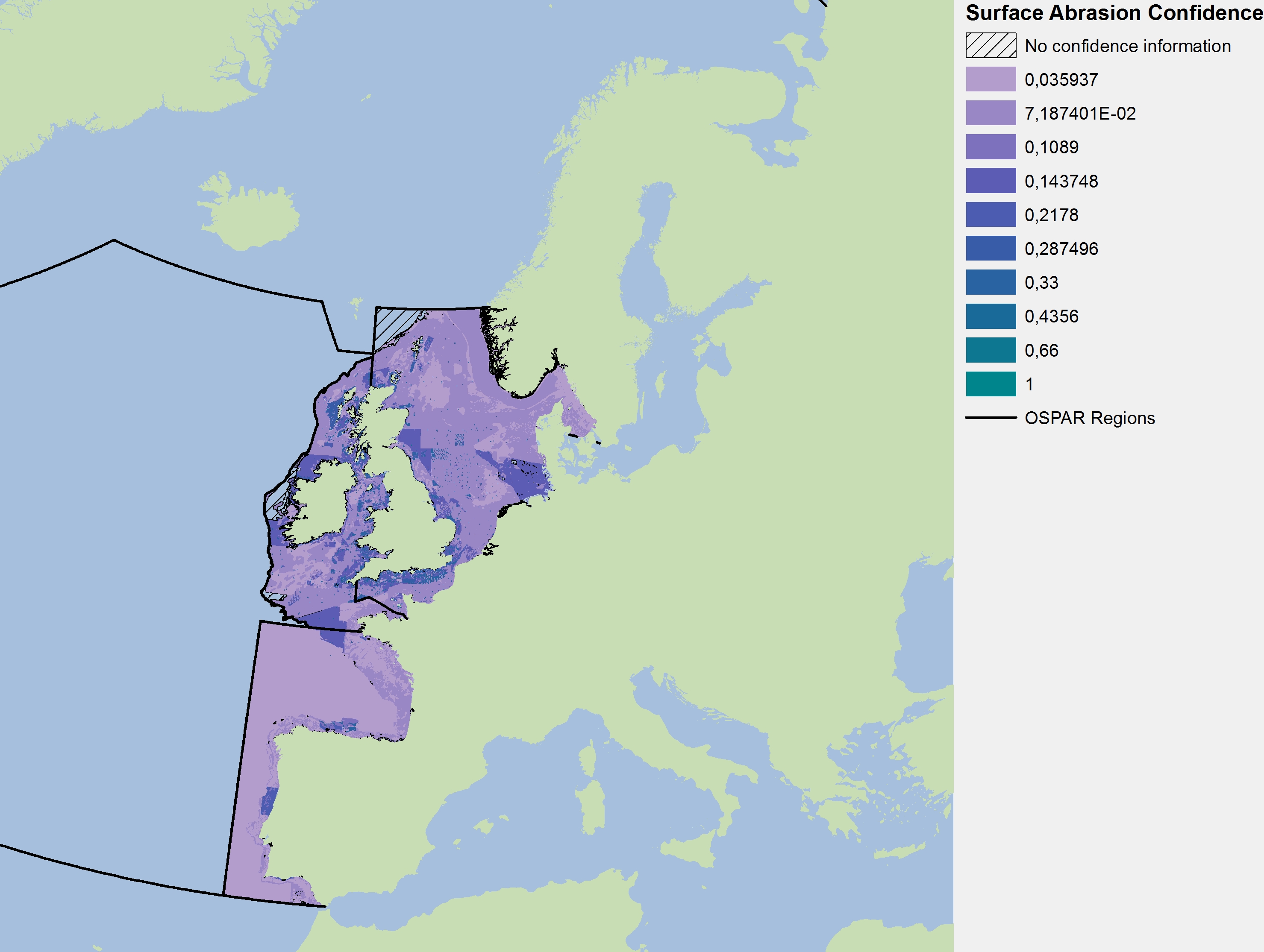
Figure q: Spatial distribution of confidence assessments for the physical damage indicator
Conclusion
L’évaluation couvre la période de 2010 à 2015. Elle révèle que jusqu’à 86% des cellules de la grille évaluées dans la mer du Nord au sens large et les mers Celtiques présentent les signes d’une certaine perturbation physique du sol marin par les engins de pêche de fond, 58% des zones révélant des perturbations d’un niveau plus élevé. Les zones évaluées dans les mers Celtiques et la Manche évaluées subissent des perturbations plus élevées que d’autres régions. L’intensité des pressions exercées durant la période d’évaluation de six ans n’est pas toujours régulière, un quart des cellules de la grille évaluées révélant une grande variabilité des pressions. Ceci est évident, en particulier, dans la mer du Nord au sens large. Les pressions de surface sont reparties uniformément dans les cellules de la grille évaluées, alors que les pressions les plus élevées exercées sur le sous-sol se trouvent le long des côtes méridionales et orientales de la mer du Nord méridionale du nord de la France au Kattegat.
On ne relève dans l’ensemble aucune tendance évidente dans les habitats ou les régions. Les résultats ne tiennent pas compte des activités de pêche benthique antérieures à 2010 qui pourraient avoir affecté des zones révélant des perturbations faibles ou qui sont soumises à des pressions exercées par d’autres activités.
On pourrait utiliser les valeurs de la répartition spatiale des perturbations en même temps que l’analyse des tendances pour orienter les discussions sur la gestion potentielle.
These results show current distribution and extent of habitat sensitivity; the overlapping fishing pressure causing surface and subsurface abrasion; and the resulting habitat disturbance. These results allow the distinction to be made between seafloor habitats of varying sensitivity that are under pressure from these types of fishing activities.
Some areas under high levels of surface and especially sub-surface abrasion, show low habitat disturbance. This could be caused by sensitive features being replaced by opportunistic and less sensitive species.
At present there are limitations due to data availability and accessibility for assessing habitat extent and distribution and associated habitat sensitivity. Combining observational data with model results is a highly effective approach in the absence of detailed survey data.
Some areas have already lost sensitive species and biotopes due to past human activities, such occurrences cannot be assessed by this Indicator and this will result in a lower disturbance score in such areas. To address this, the results of applying this Indicator will be validated using the assessment results from other benthic condition indicators, such as the assessments on Condition of Benthic Habitat Defining Communities, including the development of reference conditions, as they become available.
The method used has been thoroughly tested and reviewed by national experts working within the OSPAR framework. It represents a realistic approach for assessing the distribution of physical disturbance across the OSPAR regions based on current knowledge and using all available evidence. However, it is important to note that the strength of any assessment is dependent on the quality of the input data and the approach to its analysis, and this will in turn dictate the power and utility of the resulting information. As it stands the method proposed gives a partial assessment of physical damage at an OSPAR regional scale focused only on physical abrasion as a result of bottom fishing.
It is also expected that disturbance matrices and the final algorithm will be calibrated in the future and, if required, modified using the results from site-scale condition indicators, not only for fishery information but also for other human activities. Use of this indicator in conjunction with other site condition indicators such as the Condition of Benthic Habitat Defining Communities indicator, which is based on the European Union Water Framework Directive (WFD) (2000/60/EC) multimetric indicators, as well as the typical species will help to improve the confidence and accuracy of the results on the distribution and levels of impacts.
Lacunes des connaissances
Le but du prochain cycle d’évaluation est de progresser dans le sens d’approches plus quantitatives. Il faudra porter une attention particulière, pour y parvenir, aux points suivants: disponibilité des données et accès aux données découlant des études des habitats; absence de données sur les petites exploitations de pêche et autres activités causant des perturbations physiques (par exemple extraction de sable et travaux de construction offshore); revue de la méthode de sensibilité; affinement du tableau des perturbations; calcul d’un indice définitif des perturbations physiques par type d’habitat et sous-région et une meilleure compréhension des impacts des divers types d’engin de pêche.
Although the indicator is particularly useful for assessing large sea areas where few data exist, it would benefit from access to more accurate, abundant and high‑quality data to improve confidence in the results. Key gaps are:
Data access:
Additional information from benthic species collected during surveys can be added to improve the quality of the results, and to improve the evidence available on the distribution of sensitivity information across the regions. This alongside access to the aggregated fisheries Vessel Monitoring System (VMS) data, especially data on metiers, being collected as part of the ongoing data calls is important to improve the accuracy of results without incurring additional costs.
Quantified impacts values:
Development of quantifiable pressure-impact relationship values are very important in order to incorporate information on other activities causing physical damage, and to assess additive effects in multi-pressure systems. Scale of fishing pressure and matrix underpinning disturbance values need to be evaluated using experimental and field studies to improve evidence on the pressure-impact-response relationships. Results from the assessment of the Condition of Benthic Habitat Communities will be used to validate and calibrate impacts calculated under this assessment.
Sensitivity and disturbance data:
The evidence base can be improved if more information on the resilience and resistance of biotopes, or habitats at European Nature Information System (EUNIS) Levels 4 to 6 is made available and / or further studies are undertaken. Sensitivity information used in the production of the surface abrasion and sub-surface abrasion sensitivity layers was developed based on studies, literature reviews and matrices from the United Kingdom, France and Germany, it is therefore mainly relevant for the Greater North Sea and the Celtic Seas. This gap is of particular importance for the Bay of Biscay and Iberian Coast region as it is expected that the characterising species and biotopes will be slightly different from those in the Greater North Sea and Celtic Seas. The confidence of the assessment results will benefit from an increase in the availability of more accurate habitat data. As part of the European Union co-funded EcApRHA project, new information has been tested to increase the qualitative aspects of the indicator, especially for the analyses of sensitivities and disturbance, using case studies in The Bay of Biscay and Iberian Coast. These results, alongside data and information generated by other European Union projects have been incorporated within the methodology for the next assessment cycle. A review of the sensitivity method should also be undertaken; in particular, the relevance of incorporating recoverability aspect into the assessment and when it may be more appropriate to factor it into the temporal trend analysis and to management actions (such as priorities for habitats with very long recovery times).
Calculation of an index per region and habitat type:
The final outputs of this model are levels of disturbance per habitat type across a region. These levels of disturbance are amalgamated into a ‘Physical Damage Index‘ value for each benthic habitat. However, during indicator development a formula for calculating this Index was tested and found not to deliver satisfactory results to capture temporal changes in fisheries pressures. The formula and results are not presented here as they are still under development and further testing, which will include the revision of sensitivity/pressure matrix to incorporate new data from fishing impact curves and condition indicators. Further understanding of the cumulative effects of historical damage from some human activities and in particular the effects that the continued loss of sensitive habitats could cause on the integrity and ecological function of benthic habitats needs to be investigated to allow the definition and development of reference values. Physical damage by human activities other than fisheries, will be calculated for the next assessment cycle.
Effects of other gear types:
Better understanding is needed of the effects of differing and innovative gear types (for example, SumWing trawls), which may result in a lower abrasion pressure.
Other OSPAR Regions:
At present this indicator is still being investigated for its application in Arctic Waters and the Wider Atlantic, mainly due to limited data availability within these regions. It is anticipated that data on habitat distribution and sensitivity will be included at a later stage, to allow the analysis to address the wider spatial scale and assess variations in disturbance across OSPAR regions more accurately.
BioConsult (2013): Seafloor integrity - Physical damage, having regard to substrate characteristics (Descriptor 6). A conceptual approach for the assessment of indicator 6.1.2: ‘Extent of the seafloor significantly affected by human activities for the different substrate types’. Report within the R & D project ‘Compilation and assessment of selected anthropogenic pressures in the context of the Marine Strategy Framework Directive’, UFOPLAN 3710 25 206.
Connor, D, W., Allen, J, H., Golding, N., Howell, K, L., Lieberknecht, L, M., Northern, K, O. & Reker, J, B. (2004) The Marine Habitat Classification for Britain and Ireland Version 04.05. JNCC, Peterborough ISBN 1 861 07561 8 (internet version) http://jncc.defra.gov.uk/pdf/04_05_introduction.pdf
Church N.J., Carter A.J., Tobin D., Edwards D., Eassom A., Cameron A., Johnson G.E., Robson, L.M. & Webb K.E. (2016) JNCC Recommended Pressure Mapping Methodology 1. Abrasion: Methods paper for creating a geo-data layer for the pressure ‘Physical Damage (Reversible Change) - Penetration and/or disturbance of the substrate below the surface of the seabed, including abrasion’. JNCC report No. 515, JNCC, Peterborough
Dinmore, T., Duplisea, D. E., Rackham, B. D., Maxwell, D. L. & Jennings, S. (2003). Impact of a large-scale area closure on patterns of fishing disturbance and the consequences for benthic communities. ICES Journal of Marine Science, 60, 371-380.
Eastwood, P. D., Mills, C. M., Aldridge, J. N., Houghton, C. A. & Rogers, S. I. (2007). Human activities in UK offshore waters: an assessment of direct, physical pressure on the seafloor. ICES Journal of Marine Science, 64, 453-463.).
Eigaard Ole R., Bastardie F., Breen M., Dinesen G. E. 1, Hintzen N. T., Laffargue P., Mortensen L. O., Nielsen J. R., Nilsson H. C., O’Neill F. G., Polet H., Reid D. G., Sala A., Skold M., Smith C., Sørensen T. K., Tully O., Zengin M., and Rijnsdorp A. D. (2015). Estimating seafloor pressure from demersal trawls, seines, and dredges based on gear design and dimensions. ICES Journal of Marine Science, xxxxx
EMODnet (2010) MESH Confidence Assessment Available at: http://www.emodnet-seabedhabitats.eu/default.aspx?page=1635
EMODnet (2016). "EUSeaMap 2016 Broadscale predictive habitat maps - Draft Interim outputs: http://www.emodnet-seabedhabitats.eu"
Foden, J., Rogers, S. I. & Jones, A. P. (2010). Recovery of UK seafloor habitats from benthic fishing and aggregate extraction - towards a cumulative impact assessment. Marine Ecology Progress Series, 411, 259–270.
Foden, J., Rogers, S. I. & Jones, A. P. (2011). Human pressures on UK seafloor habitats: a cumulative impact assessment. Marine Ecology Progress Series, 428, 33–47.
Halpern, B. S., Walbridge, S., Selkoe, K. A., Kappel, C. V., Micheli, F., D'Agrosa, F. et al. (2008). A Global Map of Human Impact on Marine Ecosystems. Science, 319, 948-952.
ICES (2015). Report of the Working Group on Spatial Fisheries Data (WGSFD). http://www.ices.dk/sites/pub/Publication%20Reports/Expert%20Group%20Report/SSGEPI/2015/01%20WGSFD%20-%20Report%20of%20the%20Working%20Group%20on%20Spatial%20Fisheries%20Data.pdf
Jennings, S., Alvsvag, J., Cotter, A. J., Ehrish, S., Greenstreet, S. P., Jarre-Teichmann, A., et al. (1999). Fishing effects on the northeat Atlantic shelf seas:patterns in fishing effor, diversity and sommunity structure. III. International trawling effort in the North Sea: an analysis of spatial and temporal trends. Fisheries Research, 40, 125-134.
Jennings, S., Lee, J., & Hiddink, J. G. (2012). Assessing fishery footprints and trade-offs between landings value, habtat sensitivity, and fishing impacts to inform marine spatial planning and an ecosystem approach. ICES Journal of Marine Science, 1-11.
JNCC (2011). Review of methods for mapping anthropogenic pressures in UK waters in support of the Marine Biodiversity Monitoring R&D Programme. Briefing paper to UKMMAS evdience groups. Presented 06/10/2011.
Korpinen, S., Meski, L., Andersen, J. H., & Laamanen, M. (2012). Human pressures and their potential impact on the baltic sea ecosystem. Ecological Indicators,15, 105-114.
OSPAR, (2010). Quality Status Report 2010. OSPAR Commission. London.
OSPAR (2016) Intermediate Assessment 2017 Resources, http://www.ospar.org/work-areas/cross-cutting-issues/intermediate-assessment-2017-resources, Accessed online: 01/06/2016
Schroeder, A., L. Gutow & M. Gusky (2008): FishPact. Auswirkungen von Grundschleppnetzfischereien sowie von Sand- und Kiesabbauvorhaben auf die Meeresbodenstruktur und das Benthos in den Schutzgebieten der deutschen AWZ der Nordsee (MAR 36032/15). Report for the Bundesamt für Naturschutz.
Tillin, H.M., Hull, S.C. & Tyler-Walters, H (2010): Development of a Sensitivity Matrix (pressures-MCZ/MPA features). Defra Contract No. MB0102 Task 3A, Report No. 22. http://jncc.defra.gov.uk/pdf/MB0102_Sensitivity_Assessment%5B1%5D.pdf
Tillin, H. & Tyler-Walters, H., (2014): Assessing the sensitivity of subtidal sedimentary habitats to pressures associated with marine activities - Phase 1 Report, JNCC Report 512. http://jncc.defra.gov.uk/page-6790