

Répartition des tailles dans les communautés halieutiques
D4 - Réseau trophique marin
D4.2 - Proportion des espèces sélectionnées au sommet du réseau trophique
Message clé:
La longueur typique permet de mesurer la structure des tailles des communautés halieutiques et d’élasmobranches et elle diminue lorsque la pêche exerce des pressions importantes. La longueur typique du poisson démersal évalué, bien que faible par rapport aux années 1980, se rétablit dans l’ensemble de la zone maritime OSPAR depuis 2010. Le poisson pélagique révèle dans l’ensemble des fluctuations mais aucune tendance. A l’échelle locale, on relève des divergences avec cette tendance.
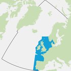
Zone Évaluée
Récapitulatif Imprimable
Contexte
L’objectif stratégique d’OSPAR, en ce qui concerne la biodiversité et les écosystèmes, est de stopper et de prévenir une perte supplémentaire de la biodiversité, de protéger et de conserver les écosystèmes et de rétablir, lorsque possible, les écosystèmes qui ont subi des impacts préjudiciables des activités de l’homme.
L’indicateur de la longueur typique est l’un de trois indicateurs du réseau trophique utilisés actuellement par OSPAR. Il représente la longueur moyenne du poisson (poisson osseux et élasmobranches) et fournit des informations sur la répartition des tailles dans les communautés halieutiques. On calcule l’indicateur à partir des données sur les captures d’espèces échantillonnées dans le cadre d’études scientifiques et exprimées en centimètres. Les communautés sont représentées par des assemblages trophiques basés sur leur habitat (groupes halieutiques): à savoir, les assemblages démersaux (c’est-à-dire espèces vivant sur le sol marin ou à proximité) et les assemblages pélagiques (c’est-à-dire espèces vivant dans la colonne d’eau).
La mortalité par la pêche limite la structure par âge des populations halieutiques, réduisant la proportion d’individus plus gros (Figure 1). On s’attend à un déclin graduel et régulier de la longueur typique en réaction à des pressions élevées exercées par la pêche. En effet la structure des tailles des assemblages halieutiques intègre les impacts des pressions exercées par la pêche durant de longues périodes. Les simulations de modèles démontrent que dans les réseaux trophiques, lorsque les interactions entre les prédateurs et les proies l’emportent sur d’autres interactions, les espèces de grande taille à des niveaux trophiques élevés (position des espèces dans le réseau trophique) sont extrêmement sensibles à la perte de diversité à des niveaux trophiques plus bas.
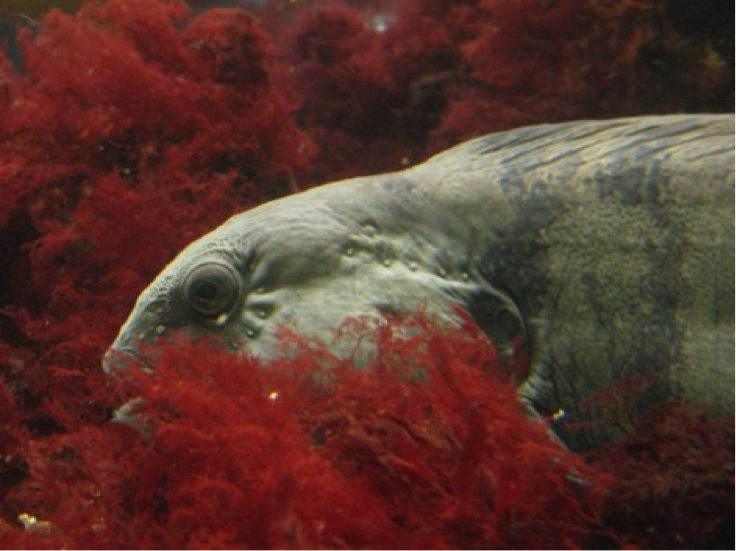
Figure 1: Loup de l’Atlantique de grande taille (avec la permission de Jim Ellis)
Fishing mortality constrains the age structure of fish communities, reducing the proportion of larger / older individuals. Fishing is also size-selective, preferentially removing larger / older fish, and therefore fundamentally affects fish community size composition. So far three indicators relating to fish size have been developed to assess impacts of fishing on healthy fish communities and the foodweb, considering similar but different parameters.
The distribution of biomass over body size (size spectra; Kerr and Dickie, 2001) is an emergent property of food webs, therefore size-based metrics that are sensitive and specific to pressures can be used as indicators of food-web structure. Jennings et al. (2007) found that body size was related to trophic level in fish in the North Sea at the community level (see also Reum et al., 2015). Barnes et al. (2010) demonstrated the relationship between fish size and trophic transfer efficiency. Riede et al. (2011) demonstrated that log-mean body size was significantly related to trophic level in marine invertebrates, and ectotherm and endotherm vertebrates using data on multiple ecosystems. Model simulations (Rossberg et al., 2008) have demonstrated that in food webs where trophic interactions dominate over other interactions, large species at high trophic levels are highly sensitive to loss of diversity at lower trophic levels (ICES, 2014a).
Fishing is a size-selective process therefore fish body size decreases during overexploitation (Boudreau and Dickie, 1992). A gradual, steady decline in Typical Length is expected in response to high fishing pressure because the size structure of the community integrates the impacts of fishing pressure over long periods of time (Rossberg, 2012; Fung et al., 2013). Processes related to rising sea temperature also serve to reduce body size of fish (Daufresne et al., 2009; Gibert and DeLong, 2014). The indicator can respond to pressures on the marine environment that impact individual fish directly (entrapment activities) or indirectly (through change in their seabed or pelagic habitat, primary production and food-web interactions). Although species are combined within the habitat-based feeding assemblages, it is possible to compute the indicator for each species individually.
The indicator is aggregated at the survey level within each region assessed and complemented by sub-divisional analyses at a scale appropriate to pressures and habitats that can be highly localised. Sub-divisional metrics are aggregated through a weighted average where those weights are given by the total surveyed biomass of relevant assemblage in each sub-division.
The Typical Length (TyL) is the weighted geometric mean length of fish, with weights given by the standardised catch rate of individuals in an area and defined as follows:
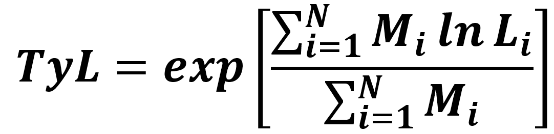
Formula a. Typical Length indicator
where Mi is the body mass (standardised to kilogrammes per unit area fished) of the i-th fish with length Li (in units of centimetres) in a sample of N fish.
Data for this indicator come from scientific fisheries surveys, which ideally sample the entire fish community but in practice do not. The indicator requires that surveys are conducted at regular intervals (e.g. annually) in the same area with a standard fishing gear. Sufficiency of available sample sizes can be judged using re-sampling techniques (Shephard et al., 2012, Lynam and Rossberg, 2017). The absolute biomass of individuals in length classes present in the environment is not recorded directly by surveys, rather observations are made from samples with detection error (including many false negatives). The detection error is further complicated by differing catchabilities over length classes and species such that the relative abundance between species and length classes observed is survey specific. Where available, catchability estimates can be used to attempt to correct for this component of the systematic measurement error (e.g. Fraser et al., 2007). However, such estimates are sparse in the scientific literature and prone to great uncertainty. In future, the recent catchability corrections estimated by Walker et al. (2017) could be considered. Alternatively, model-based estimates of absolute species abundance can be used to rescale observed abundances, but here model uncertainty is also great (ICES, 2014b). For simplicity, Typical Length is defined with reference to a particular sampling design with a varying limitation to the size range sampled by fishing gear. For each survey, this indicator is calculated for sub-divisions that represent different habitats and communities, where possible.
The data are collected under the national programmes and the Data Collection Framework (EC, 665/2008). Currently, the most important data sources for Typical Length are those groundfish surveys that are conducted through the International Council for the Exploration of the Sea (ICES). The International Bottom Trawl Survey (IBTS) programme in the Greater North Sea, Celtic Seas, and Bay of Biscay and Iberian Coast is particularly important since the trawl is a general-purpose design aimed to catch both demersal and pelagic species. However, beam trawl surveys are more efficient at catching benthivorous species such as sole (Figure a) and acoustic surveys, supplemented with pelagic trawling, are more suitable for pelagic species such as mackerel (Figure b) and time series of Typical Length from such surveys may be preferable should sufficient length sampling of fish be made.
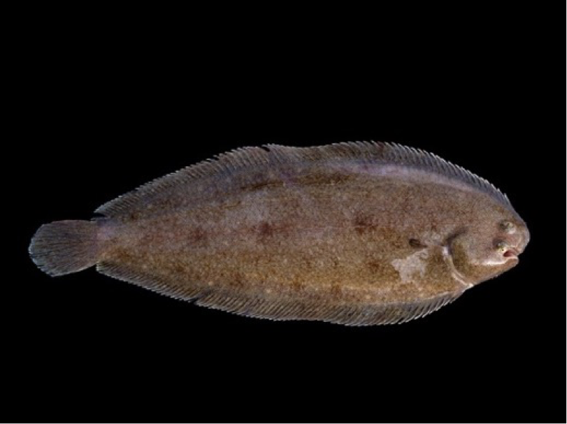
Figure a: Common sole (Solea solea) (courtesy of Hans Hillewaert)
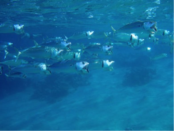
Figure b: Atlantic Mackerel (Scomber scombrus) (courtesy of Jacek Lesinowski)
Data Used and Quality Assurance
The assessment draws on raw data from the ICES database of groundfish surveys (DATRAS, www.ices.dk/marine-data/data-portals/Pages/DATRAS.aspx). These data have been quality controlled by OSPAR as part of this assessment process to generate a data product for assessment purposes. Time series of Typical Length for fish and elasmobranchs are derived from each available groundfish survey, where the community is separated into demersal and pelagic habitat-based feeding assemblages.
Time series of Typical Length by assemblage were determined for 20 surveys carried out across four separate sub-regions: the Greater North Sea, Celtic Seas, Bay of Biscay and Iberian Coast, and Wider Atlantic (Table a). Ecological sub-divisions were determined for the Greater North Sea using a simplification of those strata proposed by the EU financed project Towards a Joint Monitoring Programme for the North Sea and Celtic Sea (JMP NS/CS) that took place in 2013, and building upon work in the EU VECTORS project (Vectors of Change in European Marine Ecosystems and their Environmental and Socio-Economic Impacts) that examined the significant changes taking place in European seas, their causes, and the impacts they will have on society. In other OSPAR regions, the strata from the survey design were considered appropriate to represent the ecological sub-divisions. The survey areas and sub-divisions are shown in Figure c to Figure r. Details on the hauls (samples) for each sub-division in different years has been presented in Table b to Table x.
Standard data collected on these surveys consists of numbers of each species of fish sampled in each sample, measured to defined length categories (i.e. so a fish with a recorded length of 14 cm would be between 14.00 cm and 14.99 cm in length). By dividing the species catch numbers-at-length by the area swept by the trawl on each sampling occasion, these catch data are converted to standardised estimates of fish density-at-length, by species, at each sampling location. However, the indicator is based on biomass rather than abundance, so these abundance densities have to be converted to biomass density data by applying species weight (w) at length relationships (of the form w = aLb, where a and b are species-specific parameters). Density estimates per length category per species based on biomass (kg per km2) are referred to below as catch-per-unit-area (CPUA).
These trawl-sample density-at-length estimates are averaged retaining year, species and length category information across all trawl samples within each sampling stratum (i.e. survey specific strata following the survey design, which is a rectangular grid in the Greater North Sea and generally depth-based strata elsewhere).
| Sub-region | Survey Accronym1 | Survey period |
|---|---|---|
| Greater North Sea | GNSEngBT3 | 1990–2015 |
| GNSFraOT4 | 1988–2015 | |
| GNSGerBT3 | 2002–2015 | |
| GNSIntOT1 | 1983–2016 | |
| GNSIntOT3 | 1998–2016 | |
| GNSNetBT3 | 1999–2015 | |
| Celtic Seas | CSFraOT42 | 1997–2015 |
| CSEngBT3 | 1993–2015 | |
| CSIreOT4 | 2003–2015 | |
| CSNIrOT1 | 1992–2015 | |
| CSNIrOT4 | 1992–2015 | |
| CSScoOT1 | 1985–2016 | |
| CSScoOT4 | 1995–2015 | |
| Bay of Biscay and Iberian Coast | BBIC(n)SpaOT4 | 1990–2014 |
| BBIC(s)SpaOT1 | 1993–2014 | |
| BBIC(s)SpaOT4 | 1997–2014 | |
| BBICPorOT4 | 2002–2014 | |
| CSBBFraOT42 | 1997–2015 | |
| Wider Atlantic | WAScoOT3 | 1999–2015 |
| WASpaOT3 | 2001–2014 |
1. Survey acronym convention: first two to four capitalised letters indicate the European Union Marine Strategy Framework Directive (MSFD) sub-region (BBIC: Bay of Biscay and Iberian Coast; CS: Celtic Seas; GNS: Greater North Sea; WA: Wider Atlantic). Next capitalised and lower case letters signify the country involved (Spa: Spain; Por: Portugal; Fra: France; Eng: England; Ire: Republic of Ireland; NIr: Northern Ireland; Sco: Scotland; Ger: Germany; Int: International; Net: The Netherlands).
International refers to the two international groundfish surveys carried out in the Greater North Sea under the auspices of ICES. In the Bay of Biscay and Iberian Coast sub-region, Spanish surveys are further delimited by (n) for surveys operating in the northern Iberian coast area and (s) for surveys operating in the southern Iberian coast area).
Next two capitalised letters indicate the type of survey (OT: otter trawl; BT: beam trawl). Final number indicates the season in which the survey is primarily undertaken (1: January to March; 3: July to September; 4: October to December).
2. This is a single survey that operates across both the Celtic Seas and the Bay of Biscay and Iberian Coast sub-regions, from the southern coast of the Republic of Ireland and down the western Atlantic coast of France. For assessment purposes this single survey was split into its two sub-regional components.
Data Treatment
Surveys with rectangular sampling grids (GNSIntOT1, GNSIntOT3, GNSNetBT3, GNSGerBT3, GNSFraOT4)
Catch per unit swept area (CPUA) data (kg / km2) from multiple hauls are averaged by species for each rectangular grid cell using the strata below; in the Greater North Sea these are ICES statistical rectangles, in the eastern English Channel a mini-grid (0.25° by 0.25°) is used by GNSFraOT4. The resulting rectangle-based CPUA estimates are multiplied by the area (km2) of their rectangles (using a Lambert equal area projection) to give species biomass-at-length (now measured in kg per rectangle). Sub-divisional strata level (not GNSFraOT4) estimates of biomass-at-length are given by the sum of the rectangle-based biomass-at-length estimates and corrected by a scaling factor = 1 / (proportion of the area of sub-division monitored in the survey year) (units are now tonnes per sub-division). The scaling factor correction ensures that the weighting of the strata relative to each other in each year is not altered by the sampling levels. Sub-divisional estimates of Typical Length are calculated at this point for investigating local responses of each assemblage.
Regional estimates of biomass-at-length are estimated from the sum of sub-divisions (or in the case of GNSFraOT4 by the rectangle-based estimates). Typical Length is calculated from these data to give a survey level assessment within each region.
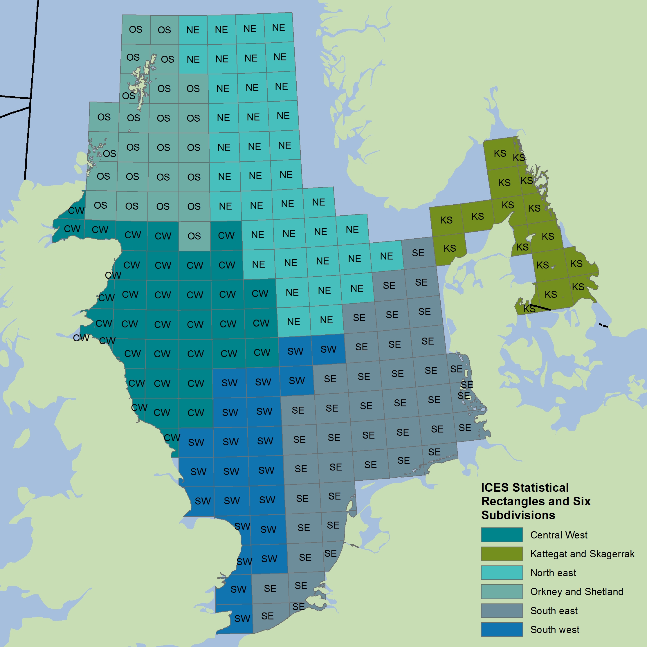
Figure c: Greater North Sea surveys with rectangular grids and sub-divisions used (note only GNSIntOT1 and GNSIntOT3 cover every sub-division appropriately)
The colours differentiate the different spatial sub-divisions used.
| Year | Central West | Kattegat & Skaggerak | North East | Orkney& Shetland | South East | South West | Total |
|---|---|---|---|---|---|---|---|
| 1983 | 64 | 33 | 62 | 35 | 140 | 42 | 376 |
| 1984 | 69 | 36 | 82 | 56 | 159 | 51 | 453 |
| 1985 | 81 | 31 | 94 | 65 | 179 | 61 | 511 |
| 1986 | 70 | 38 | 91 | 65 | 201 | 57 | 522 |
| 1987 | 88 | 43 | 94 | 61 | 187 | 58 | 531 |
| 1988 | 65 | 35 | 87 | 55 | 114 | 45 | 401 |
| 1989 | 64 | 42 | 90 | 38 | 147 | 43 | 424 |
| 1990 | 68 | 41 | 85 | 43 | 101 | 38 | 376 |
| 1991 | 69 | 37 | 99 | 46 | 123 | 47 | 421 |
| 1992 | 63 | 42 | 77 | 38 | 79 | 39 | 338 |
| 1993 | 53 | 40 | 75 | 49 | 110 | 40 | 367 |
| 1994 | 71 | 43 | 79 | 37 | 81 | 46 | 357 |
| 1995 | 64 | 44 | 76 | 28 | 79 | 41 | 332 |
| 1996 | 61 | 45 | 71 | 40 | 70 | 37 | 324 |
| 1997 | 63 | 42 | 80 | 38 | 88 | 43 | 354 |
| 1998 | 69 | 41 | 76 | 46 | 113 | 51 | 396 |
| 1999 | 69 | 42 | 73 | 37 | 83 | 47 | 351 |
| 2000 | 69 | 41 | 80 | 42 | 98 | 47 | 377 |
| 2001 | 75 | 42 | 74 | 42 | 125 | 64 | 422 |
| 2002 | 82 | 43 | 73 | 44 | 107 | 63 | 412 |
| 2003 | 81 | 42 | 73 | 46 | 99 | 65 | 406 |
| 2004 | 69 | 42 | 71 | 44 | 89 | 52 | 367 |
| 2005 | 73 | 46 | 72 | 46 | 93 | 52 | 382 |
| 2006 | 73 | 41 | 73 | 45 | 93 | 49 | 374 |
| 2007 | 63 | 42 | 67 | 40 | 90 | 46 | 348 |
| 2008 | 65 | 42 | 68 | 47 | 99 | 43 | 364 |
| 2009 | 64 | 42 | 76 | 45 | 98 | 44 | 369 |
| 2010 | 70 | 41 | 71 | 47 | 98 | 48 | 375 |
| 2011 | 67 | 39 | 68 | 44 | 98 | 49 | 365 |
| 2012 | 66 | 42 | 68 | 47 | 88 | 46 | 357 |
| 2013 | 65 | 42 | 66 | 47 | 84 | 49 | 353 |
| 2014 | 61 | 39 | 43 | 36 | 81 | 45 | 305 |
| 2015 | 64 | 42 | 66 | 47 | 82 | 48 | 349 |
| 2016 | 64 | 44 | 63 | 41 | 79 | 43 | 334 |
| Year | Central West | Kattegat & Skaggerak | North East | Orkney & Shetland | South East | South west | Total |
|---|---|---|---|---|---|---|---|
| 1998 | 54 | 40 | 54 | 31 | 58 | 31 | 268 |
| 1999 | 71 | 42 | 77 | 50 | 77 | 35 | 352 |
| 2000 | 68 | 75 | 46 | 82 | 38 | 309 | |
| 2001 | 58 | 41 | 77 | 41 | 74 | 37 | 328 |
| 2002 | 60 | 42 | 75 | 47 | 73 | 33 | 330 |
| 2003 | 60 | 42 | 70 | 42 | 70 | 35 | 319 |
| 2004 | 66 | 42 | 74 | 48 | 71 | 35 | 336 |
| 2005 | 54 | 42 | 80 | 43 | 73 | 35 | 327 |
| 2006 | 60 | 41 | 69 | 43 | 72 | 35 | 320 |
| 2007 | 55 | 40 | 69 | 46 | 66 | 35 | 311 |
| 2008 | 54 | 40 | 69 | 39 | 79 | 34 | 315 |
| 2009 | 54 | 41 | 45 | 35 | 63 | 34 | 272 |
| 2010 | 58 | 41 | 71 | 46 | 60 | 32 | 308 |
| 2011 | 58 | 43 | 73 | 44 | 66 | 34 | 318 |
| 2012 | 56 | 41 | 70 | 38 | 64 | 35 | 304 |
| 2013 | 56 | 40 | 75 | 46 | 54 | 33 | 304 |
| 2014 | 58 | 42 | 75 | 42 | 63 | 34 | 314 |
| 2015 | 60 | 43 | 74 | 46 | 69 | 35 | 327 |
| 2016 | 66 | 45 | 87 | 51 | 69 | 39 | 357 |
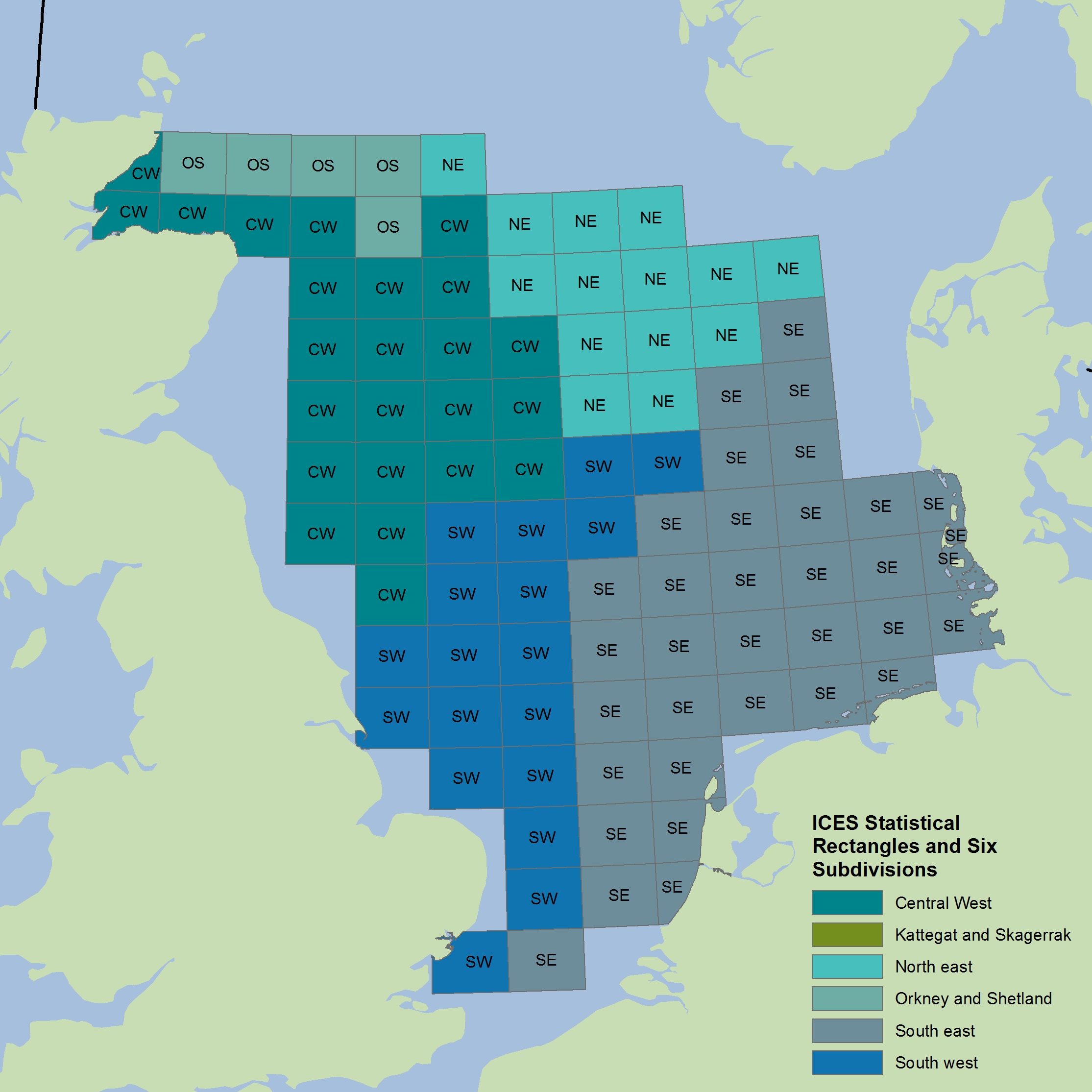
Figure d: Spatial coverage by the Netherlands groundfish survey
The colours differentiate the different spatial sub-divisions used.
| Year | Central West | North East | Orkney & Shetland | South East | South West | Total |
|---|---|---|---|---|---|---|
| 1999 | 21 | 11 | 2 | 93 | 18 | 145 |
| 2000 | 21 | 12 | 2 | 92 | 19 | 146 |
| 2001 | 21 | 12 | 4 | 83 | 10 | 130 |
| 2002 | 22 | 11 | 2 | 93 | 19 | 147 |
| 2003 | 21 | 10 | 3 | 94 | 22 | 150 |
| 2004 | 21 | 10 | 4 | 97 | 19 | 151 |
| 2005 | 22 | 11 | 4 | 100 | 22 | 159 |
| 2006 | 22 | 11 | 4 | 91 | 16 | 144 |
| 2007 | 22 | 10 | 4 | 94 | 16 | 146 |
| 2008 | 21 | 12 | 3 | 82 | 14 | 132 |
| 2009 | 21 | 12 | 3 | 88 | 15 | 139 |
| 2010 | 22 | 6 | 3 | 64 | 14 | 109 |
| 2011 | 21 | 12 | 4 | 73 | 15 | 125 |
| 2012 | 22 | 11 | 4 | 94 | 21 | 152 |
| 2013 | 22 | 12 | 3 | 86 | 14 | 137 |
| 2014 | 23 | 11 | 3 | 65 | 15 | 117 |
| 2015 | 22 | 12 | 4 | 91 | 17 | 146 |
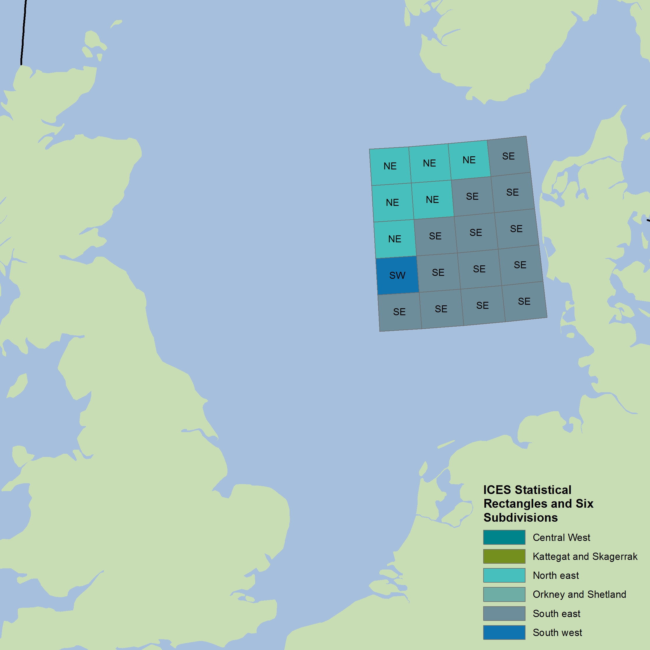
Figure e: Spatial coverage by the German groundfish survey
The colours differentiate the different spatial sub-divisions used.
| Year | North East | South East | South West | Total |
|---|---|---|---|---|
| 2002 | 13 | 28 | 3 | 44 |
| 2003 | 13 | 28 | 2 | 43 |
| 2004 | 13 | 38 | 2 | 53 |
| 2005 | 5 | 38 | 2 | 45 |
| 2007 | 13 | 32 | 2 | 47 |
| 2008 | 13 | 29 | 2 | 44 |
| 2009 | 14 | 40 | 2 | 56 |
| 2010 | 13 | 39 | 2 | 54 |
| 2011 | 13 | 40 | 2 | 55 |
| 2012 | 12 | 38 | 2 | 52 |
| 2013 | 12 | 40 | 2 | 54 |
| 2014 | 2 | 26 | 2 | 30 |
| 2015 | 13 | 40 | 2 | 55 |
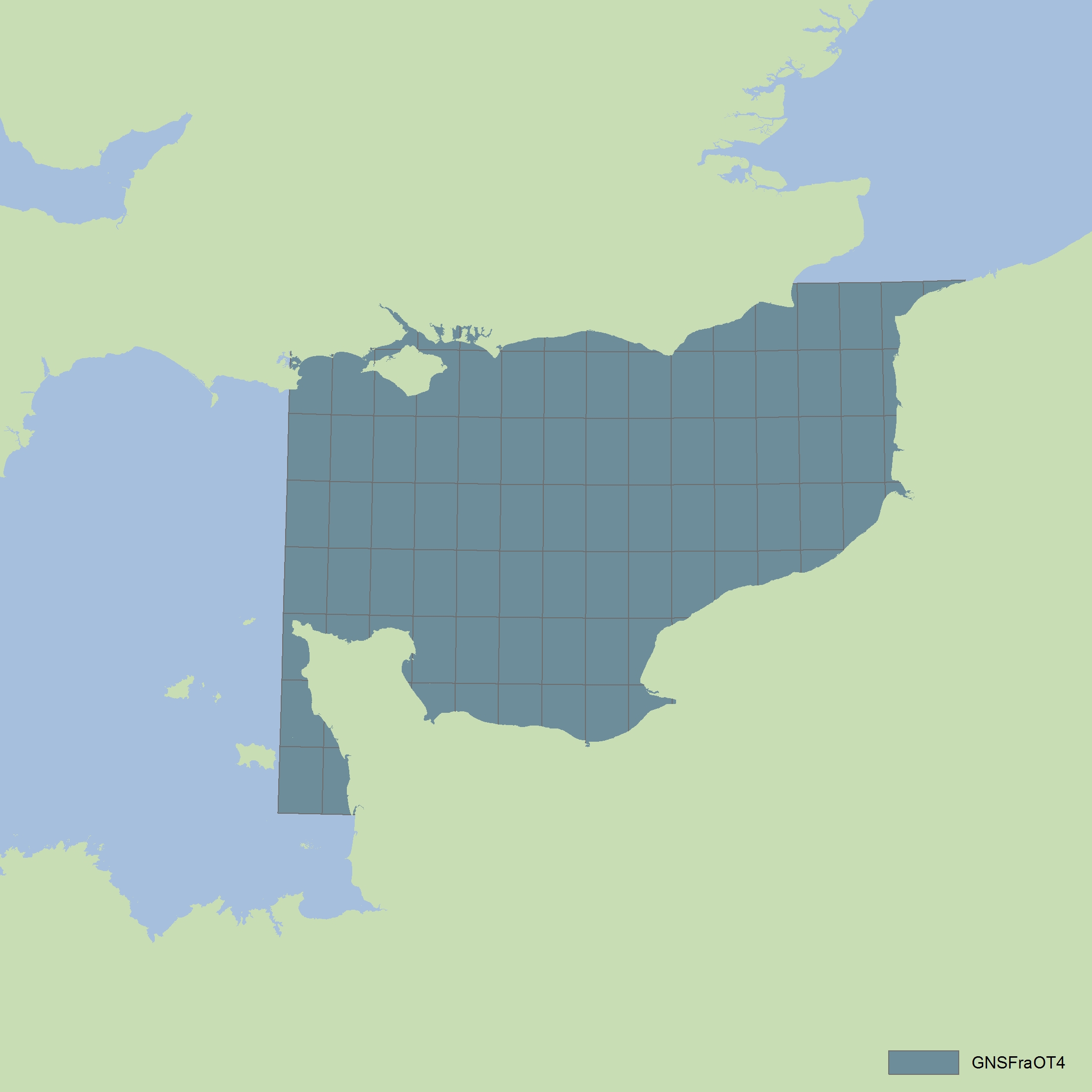
Figure f: Spatial coverage by the French channel otter trawl survey
The colours differentiate the different spatial sub-divisions used.
| Year | Total | Year | Total |
|---|---|---|---|
| 1988 | 66 | 2002 | 88 |
| 1989 | 61 | 2003 | 90 |
| 1990 | 69 | 2004 | 83 |
| 1991 | 75 | 2005 | 101 |
| 1992 | 54 | 2006 | 94 |
| 1993 | 59 | 2007 | 85 |
| 1994 | 80 | 2008 | 92 |
| 1995 | 79 | 2009 | 90 |
| 1996 | 50 | 2010 | 77 |
| 1997 | 80 | 2011 | 93 |
| 1998 | 73 | 2012 | 83 |
| 1999 | 89 | 2013 | 84 |
| 2000 | 89 | 2014 | 94 |
| 2001 | 97 | 2015 | 72 |
Surveys with irregular depth banded strata (i.e. all surveys other that those with rectangular sampling grids above)
Catch per unit swept area (CPUA) data (kg per km2) from multiple hauls averaged by species for each survey strata. Sub-divisional estimates of biomass-at-length are subsequently given by CPUA multiplied by area of the survey strata (km2, using a Lambert equal area projection). Sub-divisional estimates of Typical Length are calculated at this point for investigating local responses of each assemblage.
Regional sea estimates of biomass-at-length are estimated from the sum of sub-divisional estimates. Typical Length is calculated here for regional sea assessment.
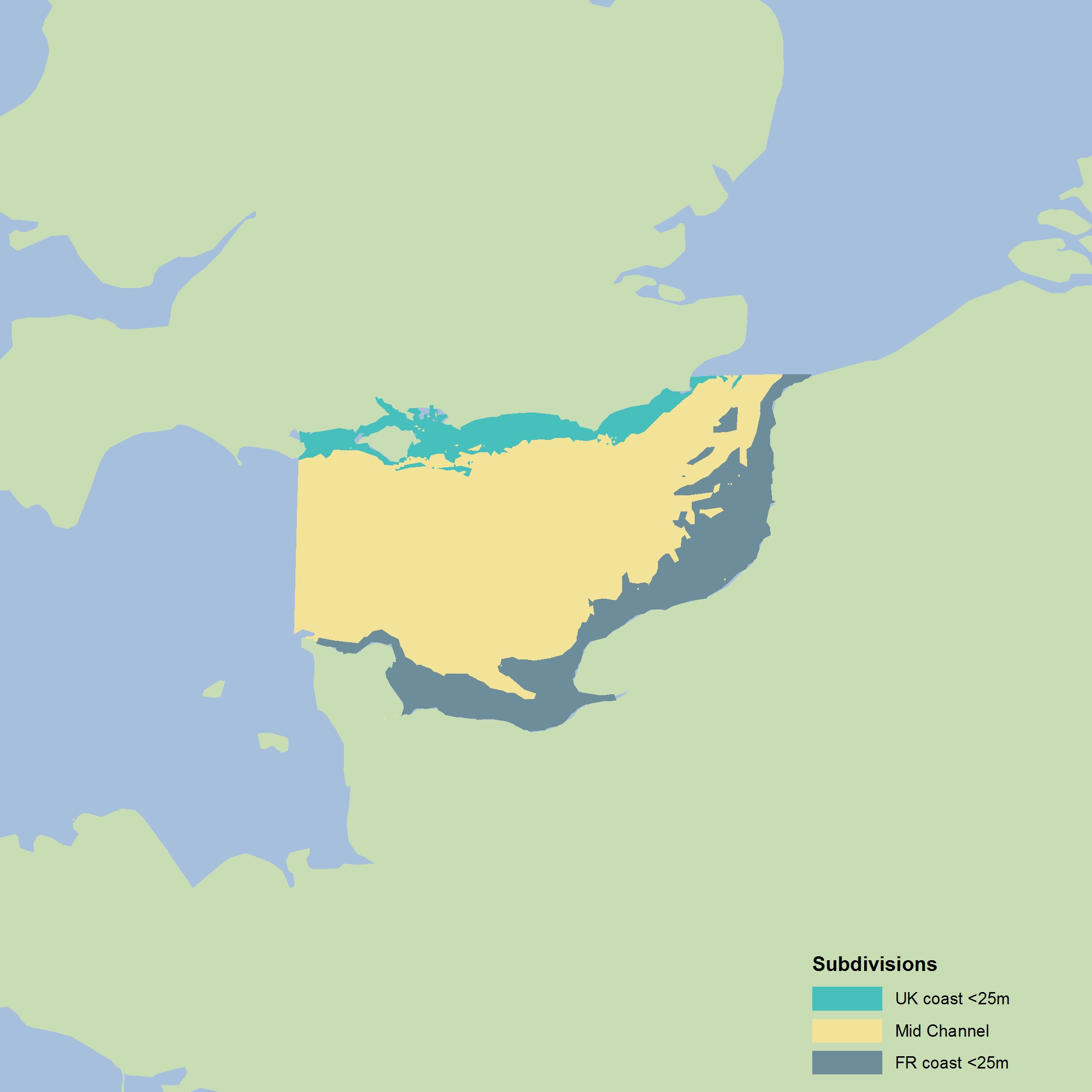
Figure g: Depth strata for GNSEngBT4
The colours differentiate the different sub-divisions used.
| Year | French coast <25 m | Mid-Channel | UK coast <25 m | Total |
|---|---|---|---|---|
| 1990 | 25 | 22 | 19 | 66 |
| 1991 | 30 | 21 | 19 | 70 |
| 1992 | 28 | 30 | 17 | 75 |
| 1993 | 28 | 25 | 19 | 72 |
| 1994 | 29 | 26 | 19 | 74 |
| 1995 | 29 | 26 | 21 | 76 |
| 1996 | 30 | 28 | 18 | 76 |
| 1997 | 29 | 24 | 20 | 73 |
| 1998 | 30 | 28 | 19 | 77 |
| 1999 | 26 | 23 | 22 | 71 |
| 2000 | 30 | 21 | 21 | 72 |
| 2001 | 29 | 29 | 33 | 91 |
| 2002 | 28 | 28 | 28 | 84 |
| 2003 | 29 | 24 | 20 | 73 |
| 2004 | 26 | 24 | 20 | 70 |
| 2005 | 22 | 17 | 19 | 58 |
| 2006 | 26 | 27 | 17 | 70 |
| 2007 | 26 | 23 | 21 | 70 |
| 2008 | 24 | 26 | 19 | 69 |
| 2009 | 25 | 25 | 21 | 71 |
| 2010 | 23 | 20 | 20 | 63 |
| 2011 | 24 | 25 | 16 | 65 |
| 2012 | 22 | 20 | 18 | 60 |
| 2013 | 23 | 24 | 17 | 64 |
| 2014 | 21 | 26 | 18 | 65 |
| 2015 | 23 | 22 | 16 | 61 |
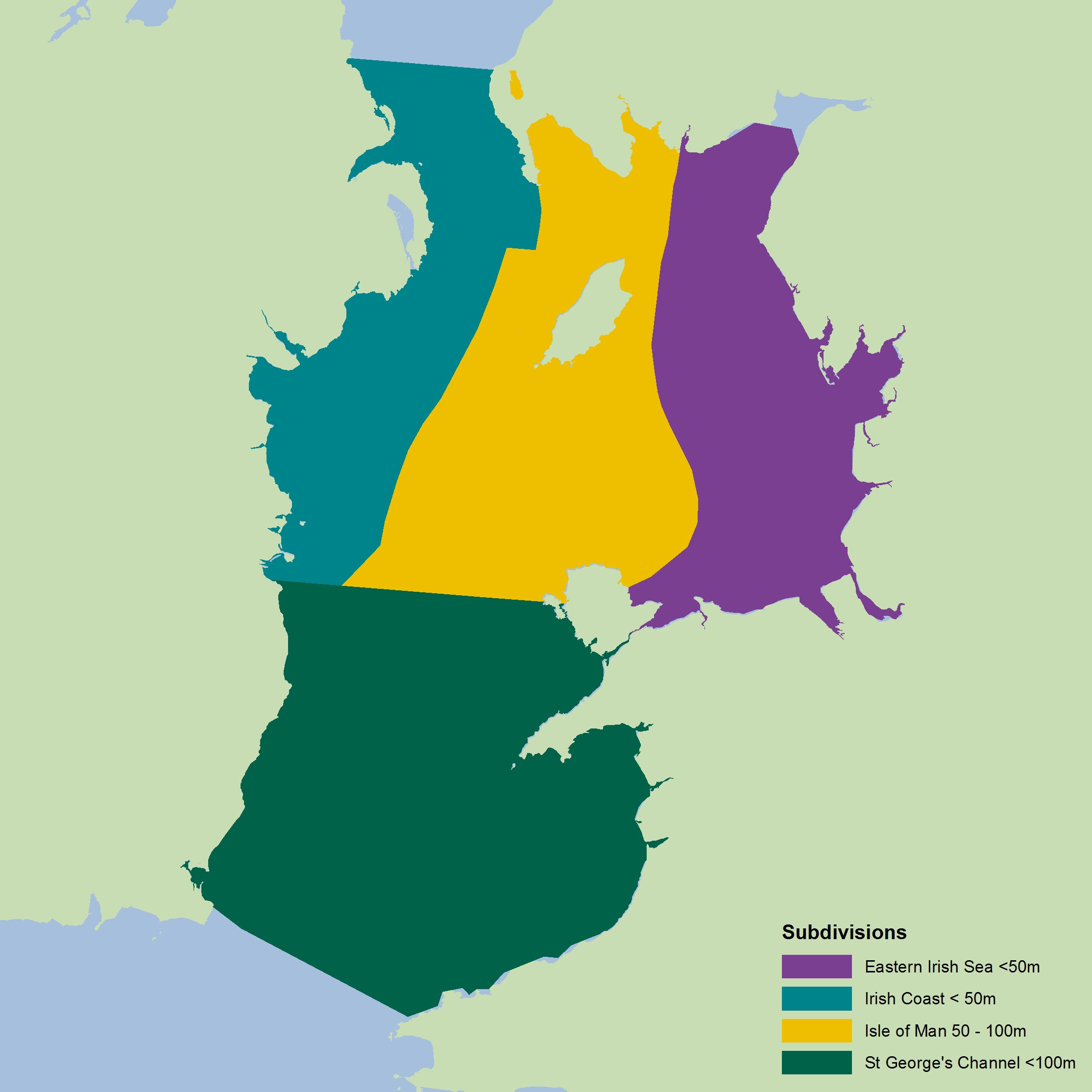
Figure h: Depth strata for Irish Sea surveys (CSEngBT3, CSNIrOT1 and CSNIrOT4) note only CSEng BT3 includes St George’s Channel
The colours differentiate the different sub-divisions used.
| Year | Irish Coast, <50 m | Isle of Man, 50–100 m | St George's Channel <100 m | Eastern Irish Sea, <50 m | Total |
|---|---|---|---|---|---|
| 1993 | 9 | 10 | 19 | 49 | 87 |
| 1994 | 6 | 14 | 15 | 30 | 65 |
| 1995 | 6 | 14 | 15 | 30 | 65 |
| 1996 | 6 | 14 | 14 | 32 | 66 |
| 1997 | 6 | 14 | 16 | 30 | 66 |
| 1998 | 6 | 13 | 15 | 30 | 64 |
| 1999 | 6 | 13 | 15 | 30 | 64 |
| 2000 | 6 | 14 | 13 | 29 | 62 |
| 2001 | 6 | 12 | 15 | 30 | 63 |
| 2002 | 6 | 13 | 16 | 30 | 65 |
| 2003 | 6 | 12 | 14 | 30 | 62 |
| 2004 | 6 | 12 | 16 | 30 | 64 |
| 2005 | 6 | 13 | 15 | 29 | 63 |
| 2006 | 6 | 12 | 15 | 30 | 63 |
| 2007 | 6 | 12 | 15 | 30 | 63 |
| 2008 | 6 | 13 | 12 | 29 | 60 |
| 2009 | 6 | 12 | 15 | 30 | 63 |
| 2010 | 6 | 12 | 16 | 30 | 64 |
| 2011 | 6 | 12 | 16 | 29 | 63 |
| 2012 | 6 | 14 | 16 | 29 | 65 |
| 2013 | 6 | 14 | 16 | 29 | 65 |
| 2014 | 6 | 14 | 14 | 29 | 63 |
| 2015 | 6 | 13 | 15 | 30 | 64 |
| Year | Irish Coast, < 50 m | Isle of Man, 50–100 m | Eastern Irish Sea, <50 m | Total |
|---|---|---|---|---|
| 1992 | 11 | 14 | 10 | 35 |
| 1993 | 18 | 16 | 10 | 45 |
| 1994 | 19 | 13 | 8 | 40 |
| 1995 | 19 | 15 | 8 | 42 |
| 1996 | 18 | 11 | 9 | 38 |
| 1997 | 19 | 14 | 7 | 40 |
| 1998 | 19 | 16 | 9 | 44 |
| 1999 | 19 | 15 | 9 | 43 |
| 2000 | 19 | 16 | 11 | 46 |
| 2001 | 19 | 17 | 10 | 46 |
| 2002 | 21 | 16 | 11 | 50 |
| 2003 | 19 | 16 | 11 | 49 |
| 2004 | 18 | 15 | 11 | 44 |
| 2005 | 19 | 11 | 8 | 38 |
| 2006 | 19 | 14 | 11 | 44 |
| 2007 | 19 | 16 | 11 | 46 |
| 2008 | 19 | 16 | 11 | 47 |
| 2009 | 19 | 15 | 11 | 47 |
| 2010 | 19 | 15 | 11 | 48 |
| 2011 | 18 | 15 | 11 | 47 |
| 2012 | 19 | 15 | 11 | 47 |
| 2013 | 19 | 16 | 11 | 49 |
| 2014 | 19 | 16 | 11 | 49 |
| 2015 | 19 | 16 | 11 | 49 |
| Year | Irish Coast, < 50 m | Isle of Man, 50–100 m | Eastern Irish Sea, <50 m | Total |
|---|---|---|---|---|
| 1993 | 18 | 16 | 10 | 44 |
| 1994 | 19 | 16 | 7 | 42 |
| 1995 | 18 | 7 | 9 | 34 |
| 1996 | 19 | 16 | 9 | 44 |
| 1997 | 19 | 16 | 9 | 44 |
| 1998 | 19 | 17 | 9 | 45 |
| 1999 | 18 | 17 | 9 | 44 |
| 2000 | 19 | 11 | 9 | 39 |
| 2001 | 19 | 15 | 11 | 48 |
| 2002 | 18 | 16 | 11 | 48 |
| 2003 | 19 | 15 | 11 | 48 |
| 2004 | 19 | 16 | 11 | 49 |
| 2005 | 18 | 16 | 11 | 48 |
| 2006 | 18 | 16 | 11 | 45 |
| 2007 | 19 | 16 | 11 | 47 |
| 2009 | 19 | 16 | 11 | 49 |
| 2010 | 19 | 16 | 11 | 49 |
| 2011 | 19 | 14 | 11 | 46 |
| 2012 | 19 | 16 | 11 | 49 |
| 2013 | 19 | 16 | 11 | 49 |
| 1992 | 24 | 12 | 8 | 44 |
| 2014 | 19 | 16 | 11 | 49 |
| 2015 | 19 | 16 | 10 | 49 |
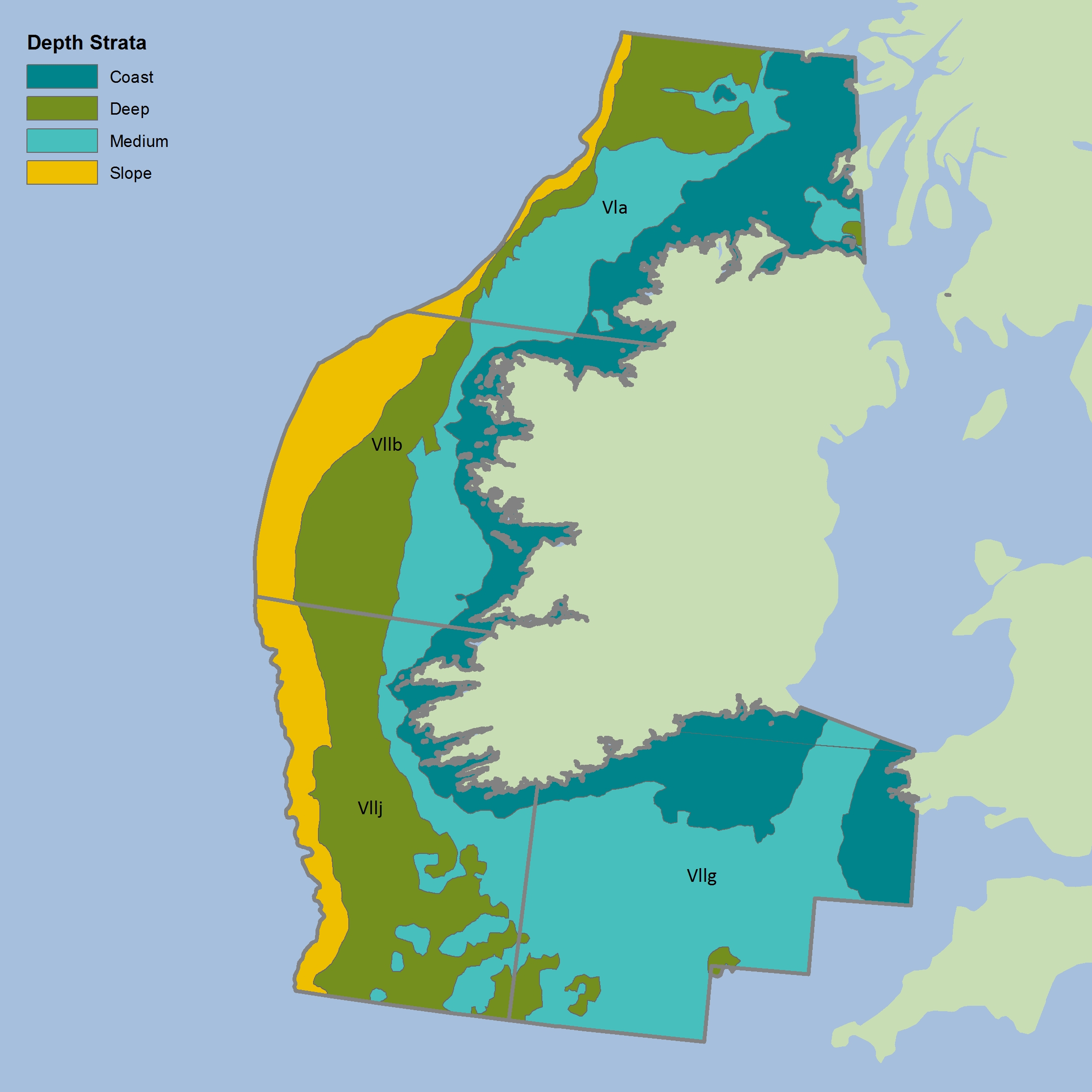
Figure i: Depth strata for CSIreOT4 survey
The colours differentiate the different sub-divisions used.
| Year | VIa_Coast | VIa_Deep | VIa_Medium | VIIb_Coast | VIIb_Deep | VIIb_Medium | VIIg_Coast | VIIg_Medium | VIIj_Coast | VIIj_Deep | VIIj_Medium |
|---|---|---|---|---|---|---|---|---|---|---|---|
| 2003 | 11 | 12 | 13 | 8 | 11 | 6 | 7 | 22 | 3 | 14 | 8 |
| 2004 | 14 | 11 | 12 | 9 | 9 | 6 | 11 | 24 | 4 | 13 | 5 |
| 2005 | 10 | 9 | 12 | 4 | 13 | 7 | 7 | 21 | 5 | 15 | 9 |
| 2006 | 19 | 11 | 12 | 7 | 9 | 8 | 10 | 26 | 4 | 17 | 8 |
| 2007 | 14 | 11 | 12 | 6 | 9 | 8 | 10 | 30 | 4 | 18 | 6 |
| 2008 | 14 | 8 | 16 | 6 | 10 | 5 | 13 | 26 | 3 | 15 | 8 |
| 2009 | 21 | 12 | 12 | 6 | 11 | 8 | 12 | 23 | 3 | 12 | 8 |
| 2010 | 14 | 13 | 13 | 6 | 13 | 8 | 14 | 34 | 4 | 19 | 10 |
| 2011 | 16 | 8 | 15 | 8 | 7 | 6 | 15 | 33 | 5 | 19 | 9 |
| 2012 | 15 | 7 | 17 | 12 | 9 | 6 | 16 | 32 | 3 | 23 | 7 |
| 2013 | 14 | 10 | 17 | 7 | 12 | 8 | 17 | 31 | 4 | 22 | 6 |
| 2014 | 15 | 11 | 12 | 5 | 13 | 7 | 17 | 33 | 4 | 19 | 7 |
| 2015 | 15 | 10 | 16 | 6 | 6 | 5 | 15 | 26 | 3 | 17 | 5 |
| Year | VIa_Slope | VIIb_Slope | VIIj_Slope |
|---|---|---|---|
| 2003 | 1 | 1 | |
| 2004 | 1 | 2 | |
| 2005 | 1 | 13 | 7 |
| 2006 | 5 | 16 | 9 |
| 2007 | 4 | 14 | 9 |
| 2008 | 4 | 17 | 10 |
| 2009 | 3 | 18 | 7 |
| 2010 | 3 | 12 | 4 |
| 2011 | 3 | 3 | |
| 2012 | 1 | 10 | 6 |
| 2013 | 2 | 12 | 5 |
| 2014 | 2 | 11 | 4 |
| 2015 | 3 | 9 | 4 |
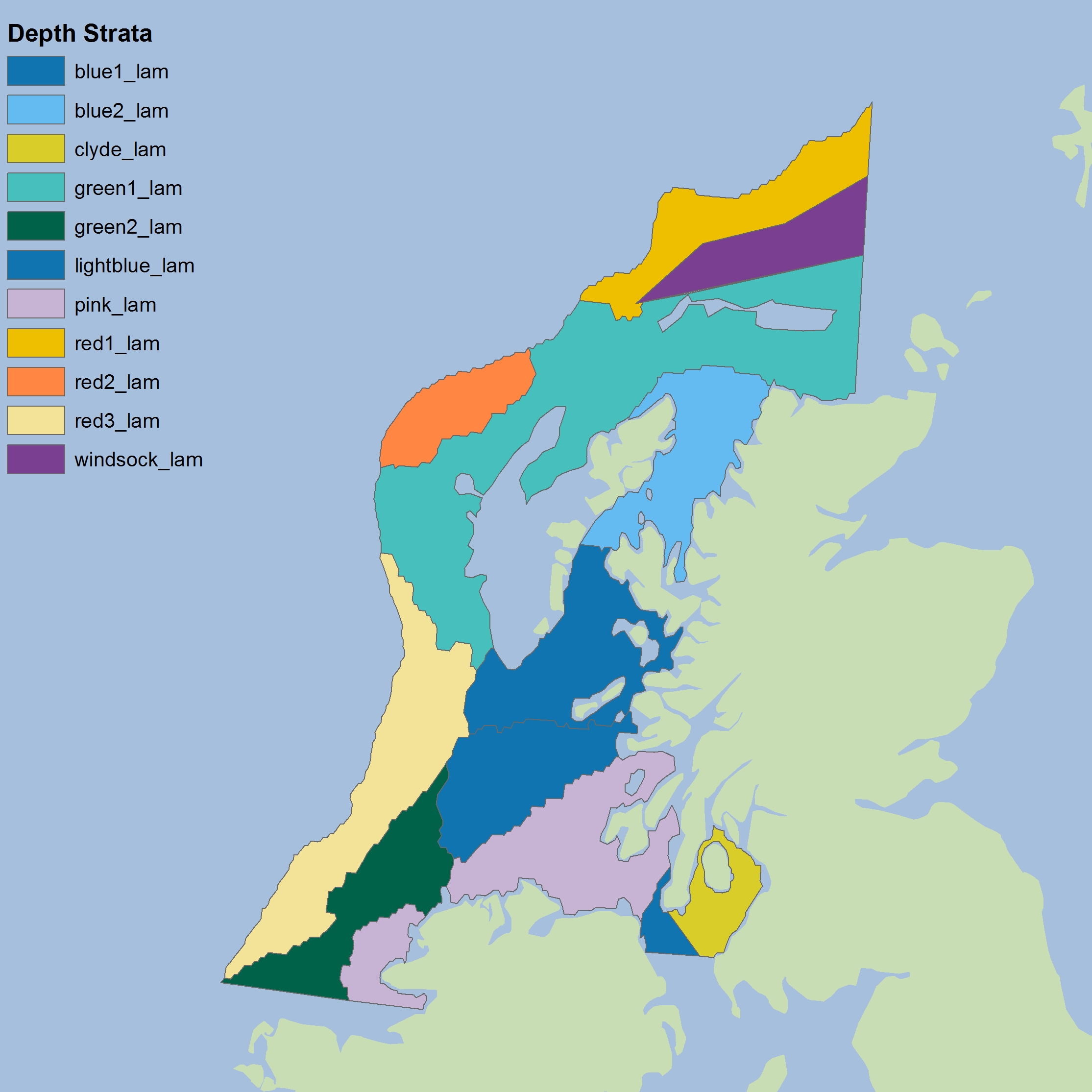
Figure j: Depth-based strata for CSScoOT1
The colours differentiate the different sub-divisions used.
| Year | blue1_lam | blue2_lam | clyde_lam | green1_lam | green2_lam | lightblue_lam | pink_lam | red2_lam | red3_lam | windsock_lam |
|---|---|---|---|---|---|---|---|---|---|---|
| 1985 | 3 | 11 | 1 | 16 | 1 | 6 | 2 | 5 | 8 | 1 |
| 1986 | 2 | 8 | 1 | 5 | 1 | 4 | 2 | 1 | 4 | 1 |
| 1987 | 2 | 10 | 1 | 8 | 1 | 4 | 2 | 2 | 5 | 4 |
| 1988 | 2 | 9 | 1 | 7 | 1 | 5 | 2 | 3 | 3 | 3 |
| 1989 | 2 | 9 | 1 | 6 | 4 | 2 | 2 | 6 | 3 | |
| 1990 | 2 | 10 | 1 | 7 | 5 | 2 | 1 | 3 | 3 | |
| 1991 | 1 | 13 | 1 | 11 | 1 | 5 | 2 | 2 | 4 | 3 |
| 1992 | 2 | 8 | 1 | 5 | 1 | 4 | 1 | 3 | 6 | 1 |
| 1993 | 2 | 10 | 1 | 6 | 1 | 5 | 2 | 3 | 4 | |
| 1994 | 3 | 11 | 1 | 7 | 1 | 4 | 2 | 1 | 5 | 1 |
| 1995 | 3 | 10 | 1 | 7 | 1 | 4 | 2 | 1 | 6 | 1 |
| 1996 | 4 | 9 | 1 | 6 | 1 | 2 | 2 | 2 | 6 | 1 |
| 1997 | 3 | 8 | 1 | 8 | 1 | 3 | 2 | 1 | 5 | |
| 1998 | 3 | 7 | 1 | 7 | 1 | 4 | 1 | 1 | 6 | 1 |
| 1999 | 2 | 12 | 2 | 8 | 1 | 5 | 2 | 2 | 6 | |
| 2000 | 3 | 14 | 1 | 7 | 1 | 4 | 2 | 2 | 6 | 1 |
| 2001 | 3 | 7 | 1 | 7 | 1 | 4 | 2 | 2 | 6 | 1 |
| 2002 | 3 | 9 | 2 | 7 | 1 | 4 | 2 | 2 | 6 | 1 |
| 2003 | 3 | 12 | 1 | 8 | 3 | 4 | 2 | 2 | 5 | 2 |
| 2004 | 2 | 10 | 1 | 7 | 1 | 5 | 2 | 2 | 6 | 2 |
| 2005 | 4 | 7 | 1 | 8 | 2 | 5 | 2 | 3 | 7 | 2 |
| 2006 | 5 | 8 | 1 | 11 | 1 | 5 | 2 | 2 | 6 | 2 |
| 2007 | 4 | 10 | 1 | 12 | 2 | 5 | 2 | 5 | 5 | 4 |
| 2008 | 3 | 8 | 1 | 9 | 2 | 7 | 2 | 4 | 7 | 2 |
| 2009 | 4 | 7 | 1 | 9 | 2 | 6 | 2 | 4 | 3 | 2 |
| 2010 | 5 | 7 | 1 | 11 | 2 | 5 | 2 | 4 | 6 | 2 |
| 2011 | 3 | 4 | 2 | 8 | 1 | 4 | 4 | 3 | 6 | 2 |
| 2012 | 5 | 6 | 2 | 13 | 2 | 7 | 3 | 2 | 4 | 1 |
| 2013 | 4 | 8 | 3 | 12 | 2 | 6 | 6 | 2 | 6 | 3 |
| 2014 | 5 | 5 | 2 | 11 | 5 | 3 | 2 | 7 | 1 | |
| 2015 | 5 | 5 | 9 | 3 | 4 | 4 | 2 | 7 | 3 | |
| 2016 | 5 | 5 | 2 | 14 | 2 | 5 | 3 | 3 | 6 | 2 |
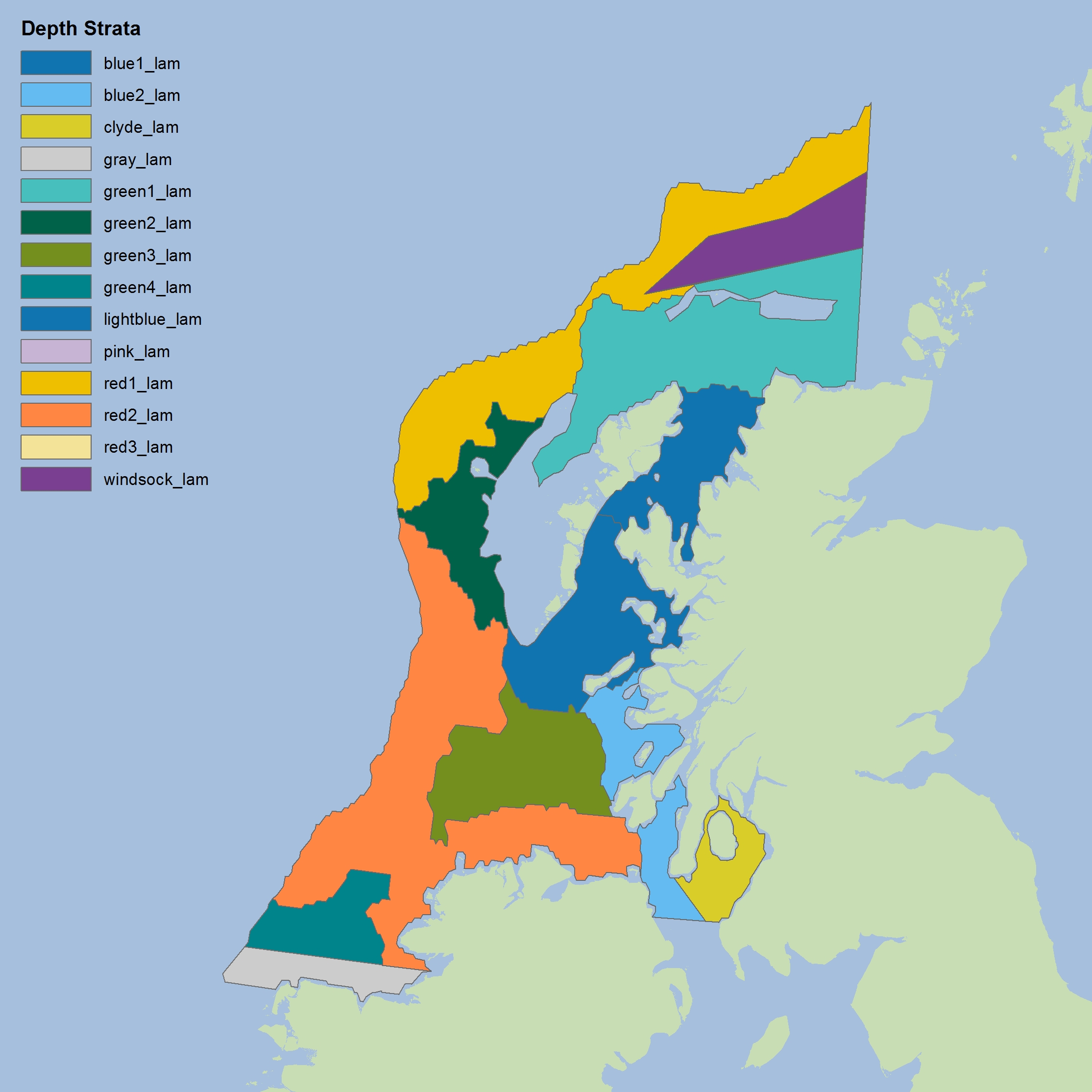
Figure k: Depth-based strata for CSScoOT4
The colours differentiate the different sub-divisions used.
| Year | blue1_lam | blue2_lam | clyde_lam | gray_lam | green1_lam | green2_lam |
|---|---|---|---|---|---|---|
| 1995 | 2 | 2 | 2 | |||
| 1996 | 3 | 7 | 3 | |||
| 1997 | 3 | 2 | 2 | 3 | 6 | 4 |
| 1998 | 2 | 2 | 2 | 3 | 5 | 4 |
| 1999 | 3 | 2 | 2 | 3 | 6 | 5 |
| 2000 | 4 | 2 | 2 | 3 | 7 | 3 |
| 2001 | 5 | 1 | 2 | 3 | 7 | 3 |
| 2002 | 5 | 1 | 2 | 3 | 10 | 3 |
| 2003 | 5 | 2 | 2 | 2 | 11 | 5 |
| 2004 | 5 | 2 | 2 | 3 | 10 | 3 |
| 2005 | 5 | 1 | 2 | 3 | 11 | 5 |
| 2006 | 5 | 2 | 2 | 11 | 5 | |
| 2007 | 6 | 2 | 2 | 3 | 15 | 4 |
| 2008 | 5 | 1 | 2 | 3 | 11 | 4 |
| 2009 | 5 | 1 | 2 | 3 | 11 | 4 |
| 2011 | 3 | 2 | 4 | 4 | ||
| 2012 | 3 | 1 | 3 | 9 | 5 | |
| 2013 | 4 | 5 | 1 | |||
| 2014 | 2 | 1 | 2 | 3 | 8 | 3 |
| 2015 | 3 | 1 | 1 | 3 | 10 | 2 |
| Year | green3_lam | green4_lam | lightblue_lam | red1_lam | red2_lam | windsock_lam |
|---|---|---|---|---|---|---|
| 1995 | 3 | 1 | 2 | 6 | ||
| 1996 | 3 | 1 | 2 | 9 | 1 | |
| 1997 | 4 | 1 | 4 | 3 | 8 | 2 |
| 1998 | 2 | 1 | 4 | 2 | 9 | 1 |
| 1999 | 1 | 1 | 5 | 1 | 8 | 2 |
| 2000 | 4 | 1 | 6 | 4 | 12 | 2 |
| 2001 | 5 | 1 | 6 | 8 | 9 | 3 |
| 2002 | 6 | 1 | 7 | 6 | 10 | 7 |
| 2003 | 5 | 1 | 7 | 5 | 9 | 4 |
| 2004 | 5 | 1 | 7 | 6 | 11 | 5 |
| 2005 | 6 | 2 | 7 | 5 | 11 | 4 |
| 2006 | 5 | 1 | 2 | 7 | 10 | 4 |
| 2007 | 5 | 2 | 7 | 7 | 15 | 5 |
| 2008 | 4 | 3 | 4 | 7 | 11 | 3 |
| 2009 | 7 | 3 | 6 | 7 | 14 | 3 |
| 2011 | 3 | 2 | 4 | 8 | 13 | 5 |
| 2012 | 8 | 2 | 3 | 8 | 15 | 3 |
| 2013 | 1 | 7 | 1 | 4 | ||
| 2014 | 5 | 1 | 7 | 10 | 11 | 4 |
| 2015 | 6 | 2 | 4 | 6 | 11 | 5 |
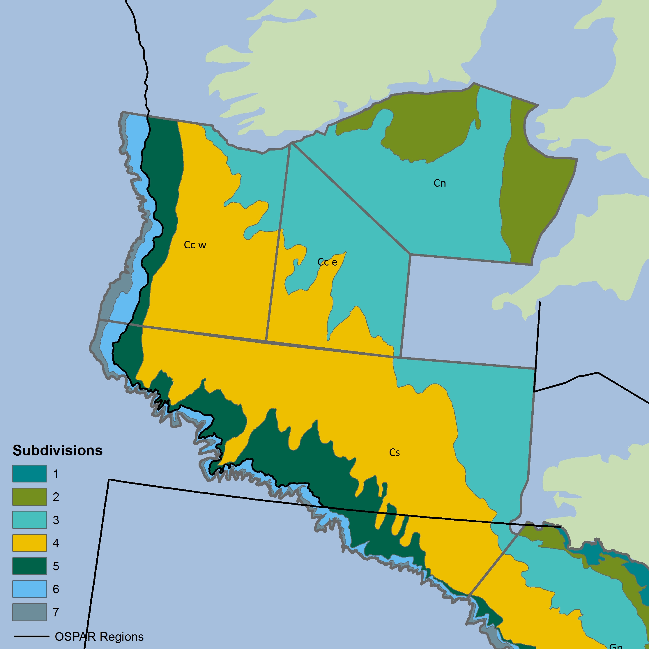
Figure l: Northern Celtic Sea strata for CSFraOT4 survey (data located above 48°N only from larger survey area) The colours differentiate the different sub-divisions used.
The colours differentiate the different sub-divisions used.
| Year | Cc3e | Cc4e | Cc4w | Cc5 | Cn2 | Cn3 | Cs4 | Cs5 |
|---|---|---|---|---|---|---|---|---|
| 1997 | 5 | 2 | 9 | 3 | 2 | 2 | 13 | 3 |
| 1998 | 9 | 1 | 9 | 3 | 2 | 4 | 12 | 6 |
| 1999 | 7 | 4 | 8 | 2 | 3 | 4 | 11 | 4 |
| 2000 | 6 | 2 | 6 | 1 | 2 | 4 | 12 | 6 |
| 2001 | 6 | 8 | 16 | 3 | 3 | 5 | 16 | 6 |
| 2002 | 4 | 5 | 14 | 4 | 4 | 4 | 16 | 7 |
| 2003 | 6 | 6 | 12 | 3 | 4 | 7 | 15 | 6 |
| 2004 | 7 | 6 | 9 | 2 | 4 | 5 | 14 | 5 |
| 2005 | 6 | 6 | 6 | 3 | 4 | 8 | 14 | 4 |
| 2006 | 5 | 6 | 9 | 4 | 4 | 4 | 9 | 3 |
| 2007 | 8 | 6 | 11 | 2 | 4 | 5 | 16 | 4 |
| 2008 | 6 | 8 | 10 | 3 | 4 | 6 | 13 | 4 |
| 2009 | 2 | 6 | 9 | 3 | 3 | 6 | 13 | 4 |
| 2010 | 4 | 1 | 11 | 3 | 3 | 4 | 12 | 5 |
| 2011 | 4 | 11 | 7 | 4 | 5 | 7 | 13 | 5 |
| 2012 | 2 | 5 | 8 | 1 | 4 | 5 | 10 | 4 |
| 2013 | 4 | 6 | 7 | 4 | 4 | 5 | 17 | 5 |
| 2014 | 7 | 4 | 12 | 3 | 4 | 5 | 12 | 6 |
| 2015 | 3 | 2 | 12 | 4 | 4 | 6 | 12 | 6 |
| Year | Cs6 | Cs7 | Cn2e | Cc3w | Cc6 | Cc7 |
|---|---|---|---|---|---|---|
| 1997 | 2 | 1 | 3 | 1 | ||
| 1998 | 2 | 3 | ||||
| 1999 | 2 | 2 | 1 | 3 | 2 | 2 |
| 2000 | 2 | 2 | ||||
| 2001 | 2 | 2 | 2 | 1 | 2 | 2 |
| 2002 | 2 | 3 | 1 | 3 | 2 | 2 |
| 2003 | 4 | 1 | 2 | 1 | 3 | 1 |
| 2004 | 1 | 3 | 3 | 2 | ||
| 2005 | 4 | 2 | 1 | 1 | 4 | 1 |
| 2006 | 1 | 2 | 1 | 3 | 3 | 1 |
| 2007 | 3 | 2 | 2 | 2 | 2 | 2 |
| 2008 | 2 | 5 | 3 | 2 | 2 | |
| 2009 | 2 | 2 | 2 | 2 | 2 | 2 |
| 2010 | 2 | 2 | 2 | 3 | 3 | 2 |
| 2011 | 4 | 3 | 2 | 3 | 1 | 2 |
| 2012 | 4 | 2 | 3 | 2 | 2 | 2 |
| 2013 | 2 | 3 | 1 | 3 | 2 | |
| 2014 | 3 | 5 | 3 | 4 | 2 | 2 |
| 2015 | 2 | 3 | 1 | 5 | 2 | 1 |
Bay of Biscay and Iberian Coast
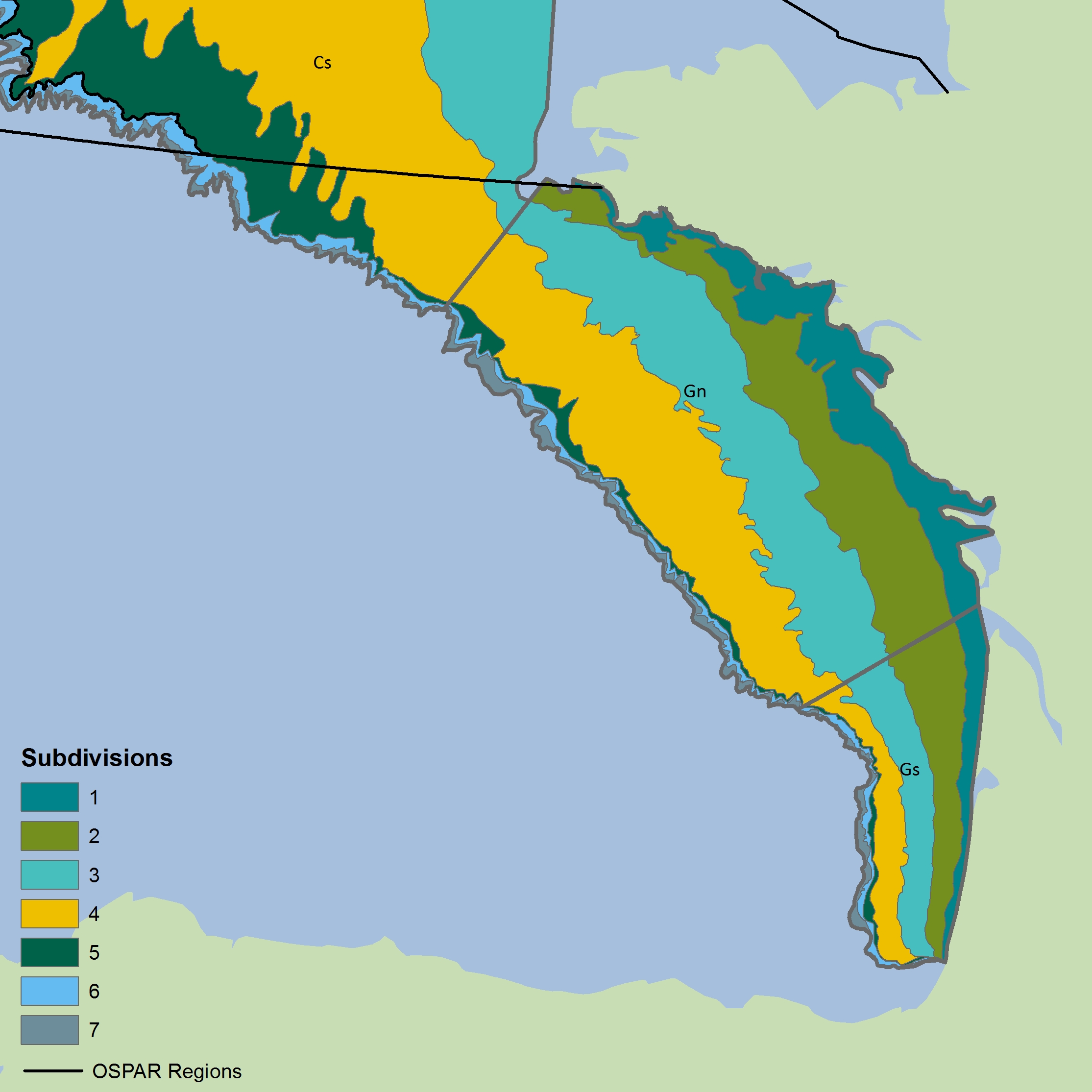
Figure m: Depth-based strata for CSBBFraOT4 (southern area, south of 48°N)
The colours differentiate the different sub-divisions used.
| Year | Gn1 | Gn2 | Gn3 | Gn4 | Gn57 | Gs1 | Gs2 | Gs3 | Gs4 | Gs5 | Gs67 |
|---|---|---|---|---|---|---|---|---|---|---|---|
| 1997 | 4 | 11 | 15 | 18 | 7 | 3 | 5 | 4 | 2 | 3 | 3 |
| 1998 | 1 | 8 | 10 | 23 | 3 | 2 | 6 | 3 | 3 | 3 | 2 |
| 1999 | 1 | 3 | 9 | 18 | 6 | 2 | 5 | 3 | 1 | 1 | 6 |
| 2000 | 2 | 4 | 18 | 19 | 7 | 2 | 3 | 3 | 3 | 5 | |
| 2001 | 6 | 18 | 22 | 6 | 2 | 2 | 3 | 3 | 2 | 4 | |
| 2002 | 3 | 3 | 18 | 18 | 7 | 2 | 6 | 2 | 3 | 3 | 4 |
| 2003 | 2 | 3 | 14 | 19 | 8 | 3 | 4 | 3 | 3 | 2 | 4 |
| 2004 | 2 | 2 | 19 | 19 | 7 | 3 | 3 | 3 | 2 | 2 | 5 |
| 2005 | 1 | 6 | 15 | 17 | 9 | 1 | 5 | 3 | 3 | 1 | 5 |
| 2006 | 2 | 4 | 15 | 16 | 7 | 3 | 3 | 3 | 2 | 2 | 5 |
| 2007 | 3 | 3 | 17 | 17 | 7 | 3 | 4 | 4 | 1 | 1 | 6 |
| 2008 | 2 | 3 | 16 | 19 | 8 | 2 | 5 | 3 | 3 | 3 | 3 |
| 2009 | 3 | 3 | 17 | 20 | 7 | 2 | 4 | 3 | 1 | 4 | 3 |
| 2010 | 2 | 5 | 18 | 18 | 7 | 2 | 4 | 3 | 1 | 2 | 6 |
| 2011 | 2 | 3 | 15 | 21 | 7 | 3 | 4 | 3 | 2 | 1 | 6 |
| 2012 | 2 | 4 | 16 | 16 | 7 | 3 | 4 | 3 | 1 | 4 | 4 |
| 2013 | 3 | 5 | 13 | 22 | 7 | 4 | 3 | 3 | 2 | 3 | 4 |
| 2014 | 3 | 5 | 16 | 20 | 5 | 2 | 5 | 3 | 2 | 3 | 4 |
| 2015 | 2 | 6 | 17 | 20 | 7 | 2 | 4 | 4 | 3 | 3 | 4 |
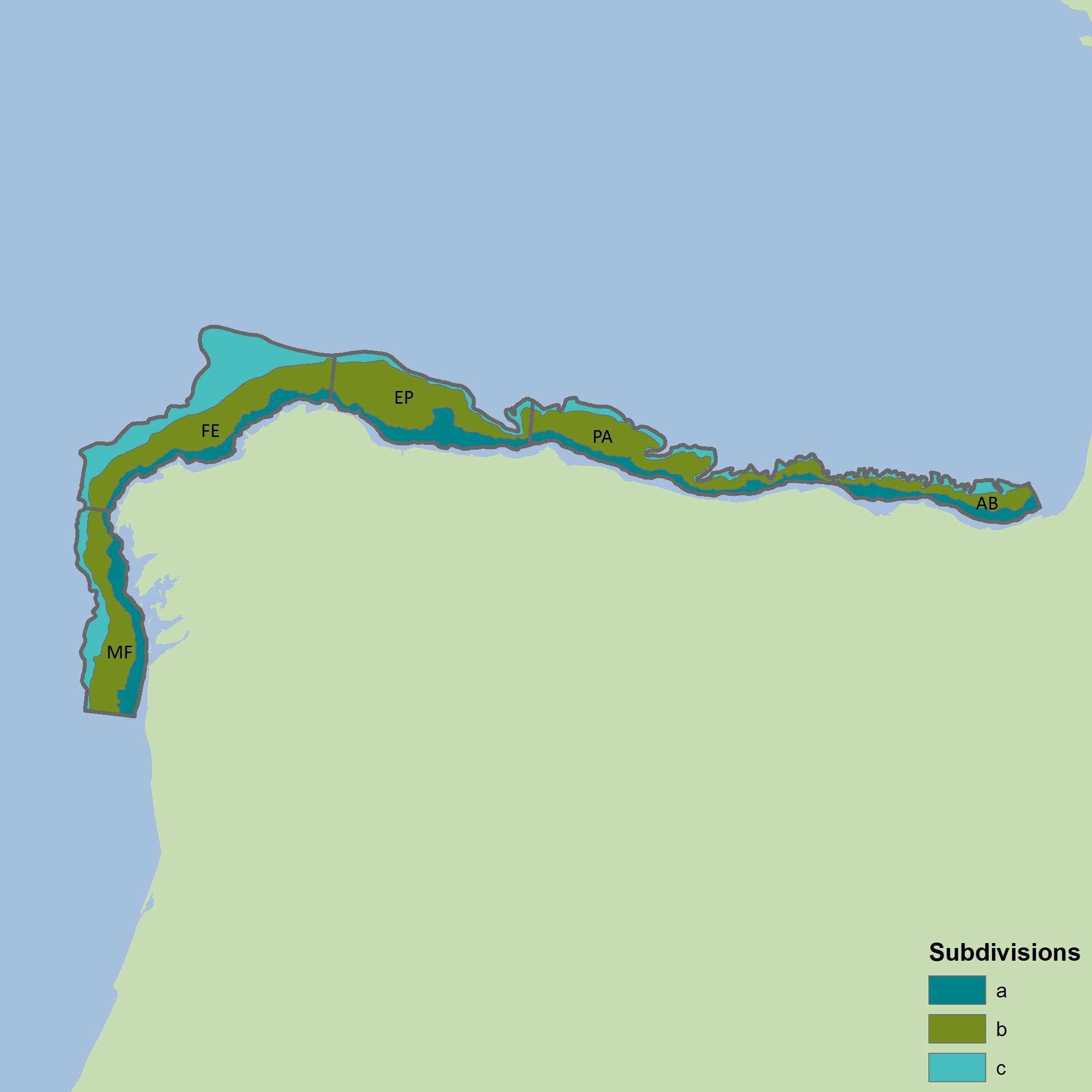
Figure n: Depth-based strata for BBICnSpaOT4
The colours differentiate the different sub-divisions used.
| Year | AB | PA |
|---|---|---|
| 1990 | 6 | 14 |
| 1991 | 11 | |
| 1992 | 2 | |
| 1993 | 13 | |
| 1994 | 14 | 9 |
| 1995 | 15 | 6 |
| 1996 | 14 | 5 |
| 1997 | 4 | |
| 1998 | 15 | 7 |
| 1999 | 15 | 9 |
| 2000 | 13 | 7 |
| 2001 | 14 | 6 |
| 2002 | 13 | 7 |
| 2003 | 13 | 6 |
| 2004 | 7 | 11 |
| 2005 | 14 | 9 |
| 2006 | 14 | 11 |
| 2007 | 14 | 10 |
| 2008 | 13 | 12 |
| 2009 | 13 | 11 |
| 2010 | 14 | 11 |
| 2011 | 14 | 9 |
| 2012 | 14 | 9 |
| 2013 | 15 | 11 |
| 2014 | 14 | 13 |
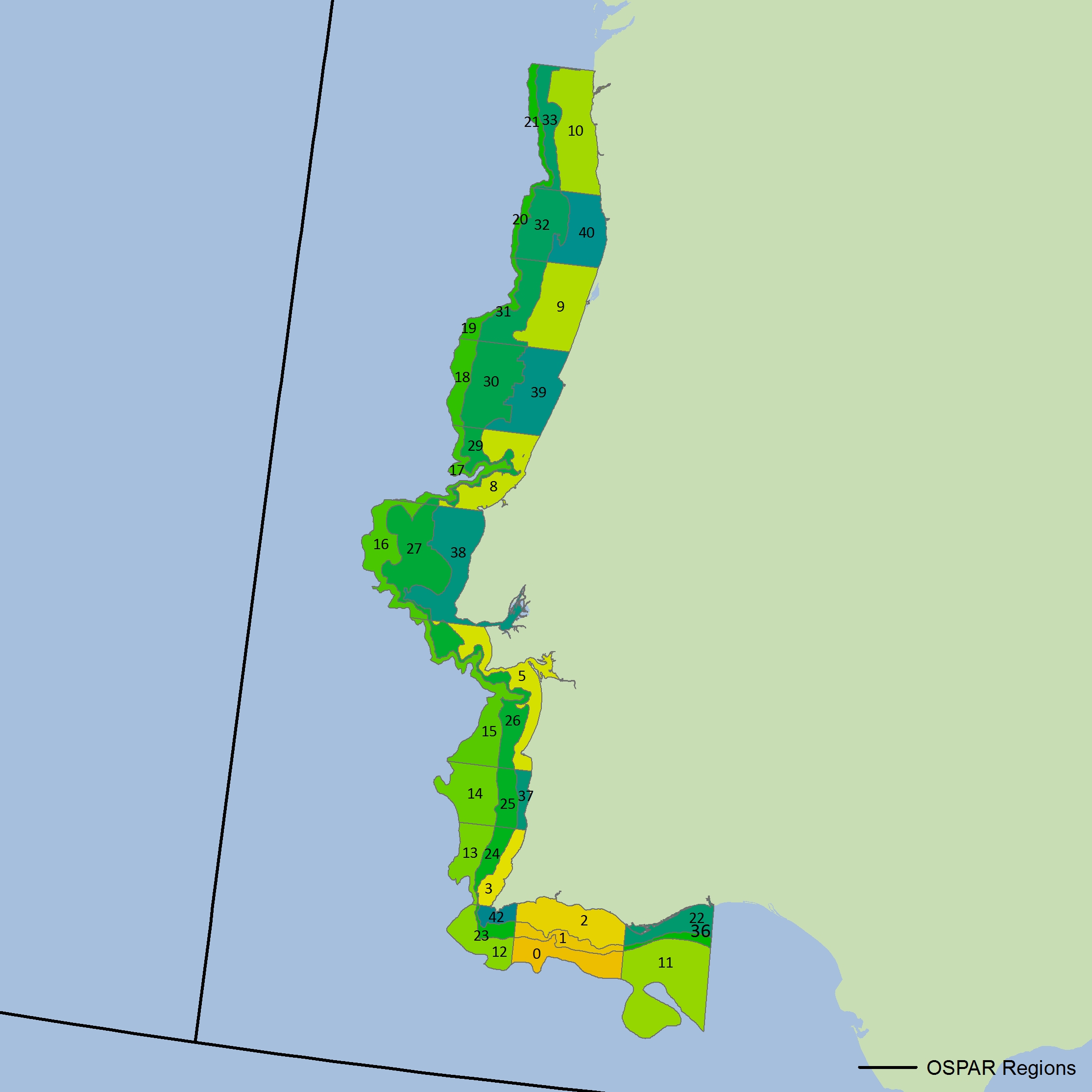
Figure o: Depth-based strata for BBICPorOT4
The colours differentiate the different sub-divisions used.
| Year | 0 | 1 | 2 | 3 | 5 | 8 | 9 | 10 | 11 | 12 | 13 | 14 | 15 | 16 | 17 | 18 | 19 |
|---|---|---|---|---|---|---|---|---|---|---|---|---|---|---|---|---|---|
| 2002 | 2 | 1 | 4 | 2 | 2 | 2 | 3 | 2 | 2 | 1 | 2 | 2 | 2 | 2 | 1 | 1 | |
| 2005 | 2 | 3 | 4 | 1 | 2 | 2 | 4 | 3 | 6 | 2 | 2 | 3 | 3 | 2 | 2 | 2 | |
| 2006 | 2 | 3 | 4 | 1 | 3 | 2 | 4 | 5 | 4 | 2 | 1 | 3 | 3 | 1 | 2 | 2 | |
| 2007 | 3 | 2 | 4 | 1 | 3 | 3 | 6 | 5 | 4 | 1 | 2 | 3 | 3 | 1 | 3 | 1 | |
| 2008 | 4 | 1 | 3 | 1 | 2 | 2 | 4 | 5 | 3 | 1 | 2 | 3 | 3 | 1 | 1 | 2 | |
| 2009 | 4 | 1 | 6 | 1 | 2 | 3 | 5 | 7 | 2 | 1 | 2 | 3 | 2 | 2 | 1 | 2 | 2 |
| 2010 | 3 | 3 | 3 | 1 | 2 | 2 | 5 | 8 | 3 | 1 | 1 | 2 | 3 | 1 | 1 | 2 | |
| 2011 | 4 | 1 | 4 | 1 | 3 | 5 | 4 | 3 | 1 | 2 | 3 | 2 | 2 | 2 | 2 | ||
| 2013 | 2 | 3 | 5 | 1 | 3 | 2 | 8 | 4 | 3 | 1 | 1 | 3 | 2 | 2 | 1 | 2 | |
| 2014 | 1 | 3 | 5 | 1 | 2 | 5 | 5 | 3 | 2 | 1 | 3 | 3 | 1 | 2 | 2 |
| Year | 20 | 21 | 22 | 23 | 24 | 25 | 26 | 27 | 29 | 30 | 31 | 32 | 33 | 36 | 37 | 38 | 39 | 40 | 42 |
|---|---|---|---|---|---|---|---|---|---|---|---|---|---|---|---|---|---|---|---|
| 2002 | 1 | 1 | 3 | 3 | 2 | 6 | 2 | 1 | 4 | 3 | 2 | 1 | 3 | 3 | |||||
| 2005 | 1 | 1 | 2 | 3 | 2 | 5 | 5 | 2 | 3 | 1 | 5 | 1 | 1 | 3 | 4 | 4 | 1 | ||
| 2006 | 2 | 1 | 3 | 4 | 5 | 4 | 1 | 3 | 1 | 5 | 2 | 1 | 1 | 6 | 3 | 1 | |||
| 2007 | 2 | 1 | 1 | 3 | 3 | 3 | 5 | 5 | 2 | 4 | 4 | 3 | 1 | 2 | 6 | 3 | |||
| 2008 | 2 | 1 | 3 | 3 | 3 | 4 | 4 | 2 | 4 | 1 | 6 | 2 | 1 | 3 | 5 | 1 | |||
| 2009 | 1 | 1 | 4 | 2 | 2 | 6 | 3 | 1 | 4 | 5 | 2 | 2 | 4 | 6 | 2 | ||||
| 2010 | 3 | 1 | 1 | 2 | 3 | 2 | 5 | 6 | 2 | 4 | 1 | 3 | 2 | 1 | 1 | 4 | 1 | 1 | |
| 2011 | 3 | 1 | 1 | 2 | 2 | 2 | 5 | 5 | 2 | 3 | 4 | 2 | 2 | 2 | 2 | 3 | 1 | ||
| 2013 | 3 | 2 | 1 | 2 | 2 | 5 | 5 | 2 | 4 | 1 | 3 | 3 | 1 | 1 | 2 | 6 | 3 | 1 | |
| 2014 | 3 | 1 | 2 | 2 | 7 | 3 | 3 | 3 | 4 | 2 | 1 | 1 | 4 | 2 | 1 |
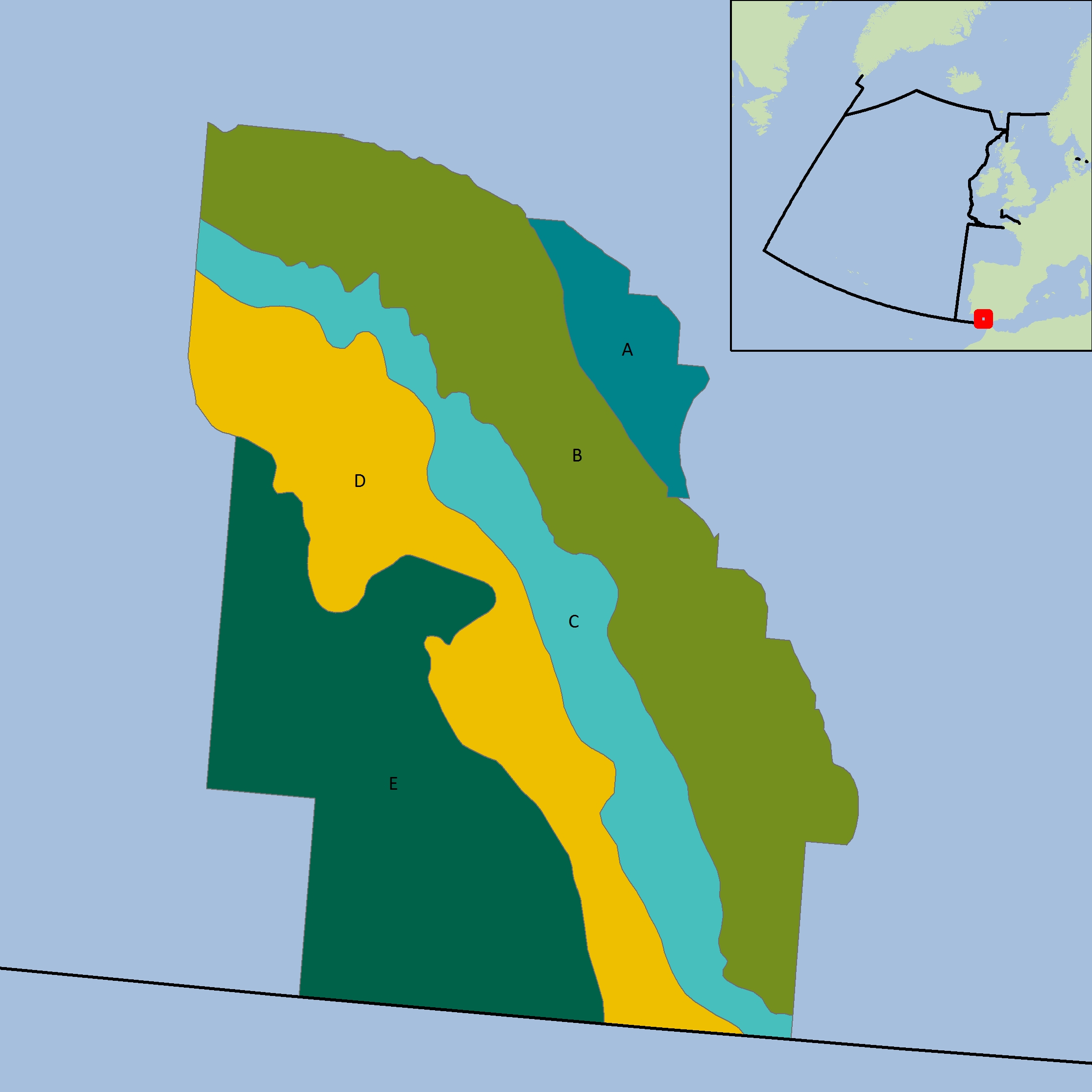
Figure p: Depth-based strata for BBICsSpaOT1 and BBICsSpaOT4
The colours differentiate the different sub-divisions used.
| Year | A | B | C | D | E | Total |
|---|---|---|---|---|---|---|
| 1993 | 2 | 5 | 5 | 5 | 7 | 24 |
| 1994 | 3 | 8 | 1 | 4 | 3 | 19 |
| 1995 | 2 | 12 | 3 | 3 | 20 | |
| 1997 | 3 | 8 | 6 | 2 | 2 | 21 |
| 1998 | 11 | 5 | 4 | 20 | ||
| 1999 | 2 | 10 | 7 | 8 | 1 | 28 |
| 2000 | 15 | 7 | 9 | 1 | 32 | |
| 2001 | 9 | 7 | 8 | 7 | 31 | |
| 2002 | 12 | 7 | 9 | 6 | 34 | |
| 2004 | 3 | 12 | 5 | 5 | 5 | 30 |
| 2005 | 12 | 6 | 8 | 6 | 32 | |
| 2006 | 1 | 11 | 7 | 7 | 6 | 32 |
| 2007 | 4 | 15 | 4 | 8 | 31 | |
| 2008 | 4 | 11 | 5 | 6 | 5 | 31 |
| 2009 | 3 | 10 | 4 | 7 | 6 | 30 |
| 2010 | 4 | 11 | 4 | 8 | 27 | |
| 2011 | 1 | 9 | 10 | 6 | 6 | 32 |
| 2012 | 3 | 8 | 5 | 5 | 2 | 23 |
| 2013 | 4 | 10 | 7 | 7 | 5 | 33 |
| 2014 | 4 | 10 | 6 | 7 | 5 | 32 |
| Year | A | B | C | D | E | Total |
|---|---|---|---|---|---|---|
| 1997 | 3 | 4 | 5 | 5 | 17 | |
| 1998 | 3 | 10 | 4 | 3 | 5 | 25 |
| 1999 | 14 | 7 | 4 | 2 | 27 | |
| 2000 | 3 | 5 | 5 | 7 | 20 | |
| 2001 | 8 | 8 | 9 | 4 | 29 | |
| 2002 | 4 | 9 | 8 | 6 | 4 | 31 |
| 2003 | 4 | 13 | 7 | 7 | 2 | 33 |
| 2004 | 4 | 13 | 6 | 7 | 3 | 33 |
| 2005 | 12 | 6 | 10 | 5 | 33 | |
| 2006 | 12 | 7 | 9 | 5 | 33 | |
| 2007 | 10 | 5 | 8 | 3 | 26 | |
| 2008 | 4 | 9 | 5 | 7 | 6 | 31 |
| 2009 | 4 | 12 | 5 | 11 | 3 | 35 |
| 2010 | 13 | 8 | 9 | 5 | 35 | |
| 2011 | 10 | 8 | 9 | 4 | 31 | |
| 2012 | 3 | 11 | 7 | 6 | 27 | |
| 2014 | 11 | 9 | 10 | 4 | 34 |
Wider Atlantic
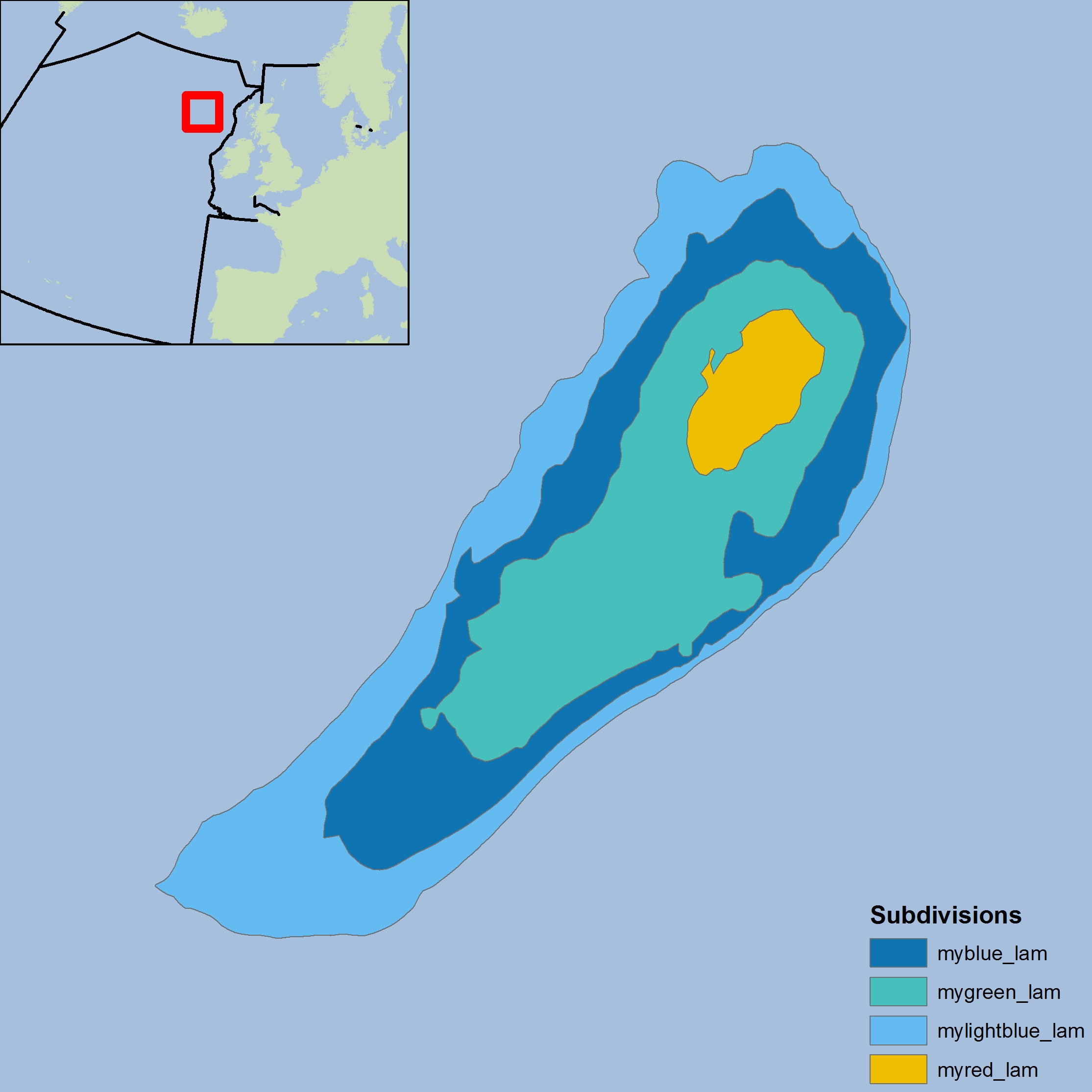
Figure q: Depth-based strata for WAScoOT3
The colours differentiate the different sub-divisions used.
| Year | myblue_lam | mygreen_lam | myred_lam | mylightblue_lam | Total |
|---|---|---|---|---|---|
| 1999 | 4 | 31 | 6 | 41 | |
| 2001 | 3 | 35 | 6 | 44 | |
| 2002 | 2 | 25 | 2 | 29 | |
| 2003 | 4 | 49 | 7 | 60 | |
| 2005 | 2 | 32 | 4 | 38 | |
| 2006 | 1 | 27 | 4 | 32 | |
| 2007 | 4 | 32 | 6 | 42 | |
| 2008 | 33 | 4 | 37 | ||
| 2009 | 4 | 34 | 3 | 41 | |
| 2011 | 8 | 19 | 5 | 5 | 37 |
| 2012 | 6 | 18 | 4 | 3 | 31 |
| 2013 | 8 | 15 | 5 | 2 | 30 |
| 2014 | 11 | 21 | 4 | 2 | 38 |
| 2015 | 9 | 21 | 4 | 5 | 39 |
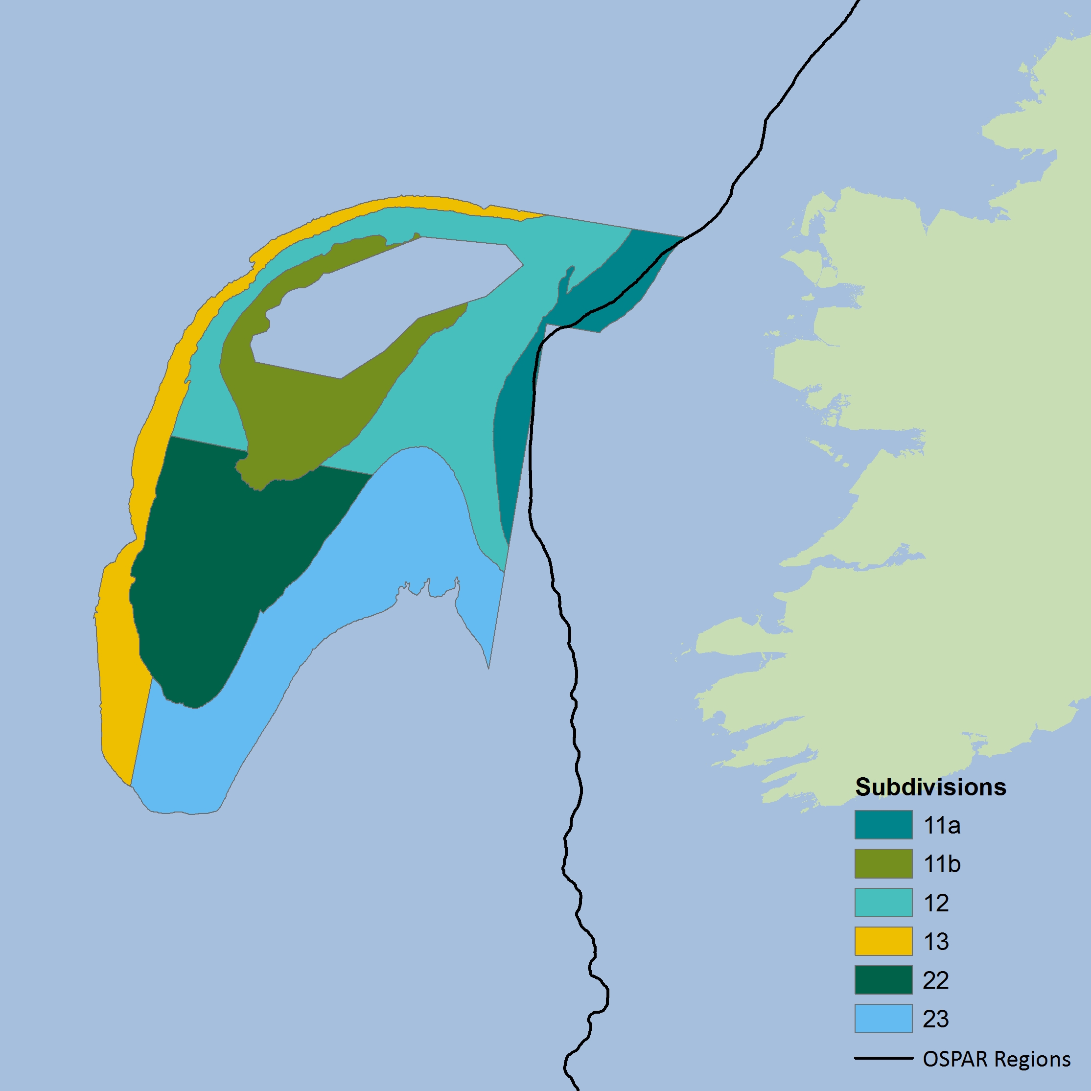
Figure r: Depth-based strata for WASpaOT3
The colours differentiate the different sub-divisions used.
| Year | 12 | 13 | 22 | 23 | 11a | 11b | Total |
|---|---|---|---|---|---|---|---|
| 2001 | 16 | 8 | 18 | 20 | 2 | 10 | 74 |
| 2002 | 18 | 5 | 17 | 20 | 6 | 10 | 76 |
| 2003 | 20 | 7 | 15 | 14 | 5 | 11 | 72 |
| 2004 | 16 | 4 | 15 | 11 | 5 | 10 | 61 |
| 2005 | 18 | 5 | 16 | 15 | 5 | 9 | 68 |
| 2006 | 19 | 6 | 15 | 15 | 5 | 10 | 70 |
| 2007 | 19 | 5 | 17 | 16 | 6 | 9 | 72 |
| 2008 | 19 | 5 | 16 | 14 | 7 | 7 | 68 |
| 2009 | 20 | 5 | 14 | 17 | 6 | 9 | 71 |
| 2010 | 17 | 9 | 17 | 16 | 6 | 5 | 70 |
| 2011 | 19 | 8 | 17 | 12 | 5 | 10 | 71 |
| 2012 | 18 | 7 | 15 | 16 | 4 | 11 | 71 |
| 2013 | 19 | 5 | 13 | 20 | 6 | 9 | 72 |
| 2014 | 19 | 7 | 14 | 17 | 7 | 8 | 72 |
Overall Assessment Basis
Where multiple surveys were available for assessment, key surveys were prioritised for assessment given the length of time series available and spatial coverage. If these measures were equal between surveys, then whichever surveyed the greatest biomass by assemblage was selected for indicator assessment. The following surveys were considered key:
Greater North Sea
GNSIntOT1 for both demersal and pelagic assemblages was selected as the key survey (preferred) for the Greater North Sea, given that it is the longest survey with the best spatial coverage. For the eastern English Channel, GNSEngBT3 was preferred for demersal assemblage given more consistent sampling here than GNSIntOT1 and GNSFraOT4. GNSFraOT4 was preferred for the pelagic assemblage in the eastern English Channel given the length of time series available.
Celtic Seas
CSScoOT1 for both demersal and pelagic assemblages was preferred over CSScoOT4 and CSIreOT4 due to length of time series. CSIreOT4 for both demersal and pelagic assemblages was preferred for sub-divisions to the west of Ireland and in the northern Celtic Sea, but not in the north where there was overlap with CSScoOT1. CSFraOT4 for both demersal and pelagic assemblages was preferred in sub-divisions of the Celtic Sea, except where overlap occurred with CSIreOT4.
CSEngBT3 for the demersal assemblage was preferred for the Irish Sea over CSNIrOT1 and CSNIrOT4 given its greater spatial coverage. CSNIrOT1 for the pelagic assemblage was preferred for the Irish Sea over CSNIrOT4 given relatively high biomass of the assemblage caught and identical coverage spatially and temporally.
Bay of Biscay and Iberian Coast
BBICsSpaOT1 for both demersal and pelagic assemblages was preferred over BBICsSpaOT4 given the length of the survey. CSBBFraOT4, BBICPorOT4 and BBICnSpaOT4 did not overlap with any other surveys.
Time-Series Assessment
In each case, the minimum value observed over the time series, prior to the last six years, was considered as a lower limit that should be avoided in future. The long-term trend in each time series (sub-division and survey level) was modelled through the application of a LOESS smoother (i.e. locally weighted scatterplot smoothing) with a simple ‘fixed span’ of one decade.
Breakpoint analyses uses data to define stable underlying periods (see Probst and Stelzenmüller, 2015). The method makes it possible to say whether there is a significant change in the time series state over time, namely whether the recent period is not significantly different from the historically observed period. The method avoids the arbitrary choice of reference periods for assessment (i.e. how many years to use to calculate an average) which can lead to subjective assessments. The shorter the period chosen, the more likely it is that noise in the data or natural fluctuations in the system are being compared against each other. However, too long a period and it could be that actual changes in state are averaged out. The minimum detectable period is defined in this analysis as three years. The analysis uses two statistical approaches: First applying the ‘supremum F test’ to establish whether a non-stationary time series or a constant period for the entire time series is more suitable. If the former, then breakpoint analysis is applied to find periods of at least three years duration.
Populations should have a size structure indicative of sustainable populations and should occur at levels that ensure long-term sustainability in line with prevailing conditions. There should be no significant adverse change in the function of different trophic assemblage levels due to human activities. Appropriate baselines for both demersal and pelagic assemblages are not currently available to determine assessment thresholds. The current assessment uses a time-series approach to identify long-term changes in state and further investigation is required to identify if reductions in the size structure of assemblages is due to human activities, food web interactions or prevailing climatic conditions.
Résultats
Les résultats de cette évaluation (Figure 2) s’appliquent au niveau de la communauté et n’identifient aucune espèce en particulier.
Mer du Nord au sens large
L’assemblage halieutique démersal évalué se rétablit à l’échelle de la mer du Nord au sens large dans son ensemble grâce aux augmentations récentes de l’indicateur de la longueur typique dans certaines sous-divisions: Orkney / Shetland, Kattegat / Skagerrak et la côte du Royaume-Uni dans la Manche. Le niveau actuel est cependant faible par rapport à la structure des tailles relevées dans les années 1980. Des zones du sud-est et du centre-ouest de la mer du Nord continuent à causer des préoccupations, les déclins à long terme ayant atteint les niveaux les plus bas relevés. L’assemblage halieutique pélagique révèle dans l’ensemble des fluctuations mais aucune tendance, à l’exception d’une diminution à long terme atteignant un niveau minimal au sud-est de la mer du Nord.
Mers Celtiques
Les études révèlent des signes mitigés au sein des mers Celtiques quant à la longueur typique de l’assemblage halieutique démersal mais des études réalisées au nord suggèrent un certain rétablissement par rapport aux faibles longueurs précédentes, des augmentations étant relevées à l’ouest de l’Ecosse. Des diminutions sont cependant évidentes dans les eaux du rebord continental à l’ouest. On retrouve le même tableau ailleurs, on relève des diminutions près de la côte irlandaise de la mer d’Irlande et dans la zone du Clyde mais des augmentations au sud de l’Irlande, à l’île de Man, dans la mer des Hébrides et dans le Minch. L’assemblage halieutique pélagique ne révèle dans l’ensemble aucune modification à long terme au niveau sous-régional. On relève cependant des augmentations au sud de l’Irlande et des diminutions dans certaines zones septentrionales, notamment dans la mer des Hébrides et les zones côtières de la mer d’Irlande et à l’ouest de l’Irlande.
Golfe de Gascogne et côte ibérique
La longueur typique de l’assemblage halieutique démersal a augmenté dans cette région à la suite d’augmentations à long terme dans les sous-divisions septentrionales des eaux du plateau à l’ouest de la France et dans les eaux côtières de la mer de Cadix. Nombre de sous-divisions à l’ouest du Portugal ont également révélé des augmentations, contrairement aux diminutions dans certaines zones du sud. L’assemblage halieutique pélagique ne révèle dans l’ensemble aucune modification à long terme. On a cependant relevé des diminutions atteignant un niveau bas par rapport à la structure des tailles relevée antérieurement dans les sous-divisions septentrionales des eaux du plateau à l’ouest de la France.
Atlantique au large
La longueur typique de l’assemblage halieutique démersal a augmenté dans le banc de Porcupine et le banc de Rockall. On a relevé des fluctuations sans modification à long terme de la structure des tailles des assemblages halieutiques pélagiques, alors que récemment (six dernières années) on a relevé une augmentation linéaire pour le banc de Porcupine.
La méthode utilisée dans cette évaluation inspire une confiance modérée / faible et la disponibilité des données inspire une confiance élevée.
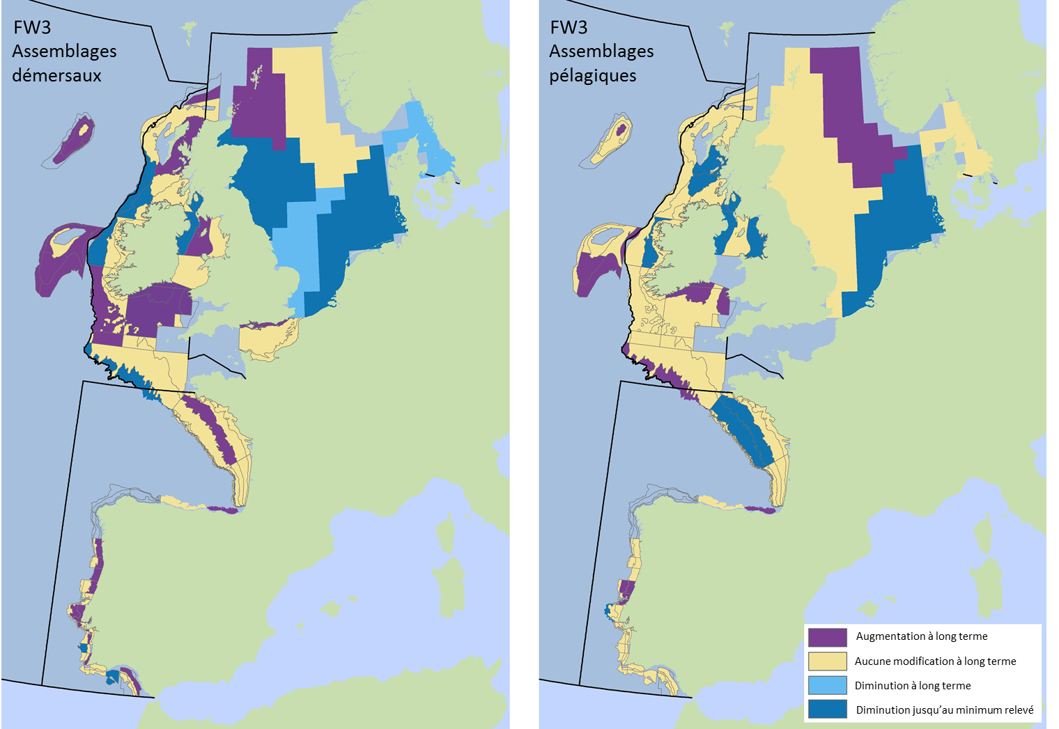
Figure 2: Profil spatial de l’indicateur de la longueur typique et séries temporelles pour les études fondamentales
La longueur typique du poisson et des élasmobranches est divisée en assemblages démersaux (à gauche) et en assemblages pélagiques (à droite) dans le cadre des sous-divisions d’études fondamentales, lorsque des données sont disponibles. La longueur de la période pour laquelle des modifications à long terme sont définies dépend des données disponibles pour l’étude, toutes les périodes considérées étant de plus de dix ans.
Figure s to Figure ay show time series for each survey sub-division. The label for the different sub-divisions is above the plot. For each figure the plot labelled ‘sea’ is a time series of the aggregated survey data for demersal and pelagic assemblages. Each mini-heading shows the p value for the supremum F test which demonstrates whether a significant long-term change is evident (the changes are shown by red dashed lines if significant, or a grey dashed line is used to show a mean level for the whole time series). Annual estimates are shown by blue circles with a fitted LOESS smooth plot (black line) with an estimate of spread shown (± 1 standard deviation). The solid horizontal blue line shows the minimum observed data point prior to the most recent six data points and two horizontal thin black lines showing the average indicator value for the first and last six years.
Greater North Sea
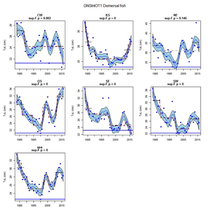
Figure s: Time series of Typical Length for each sub-division of the GNSIntOT1 survey (Demersal fish species)
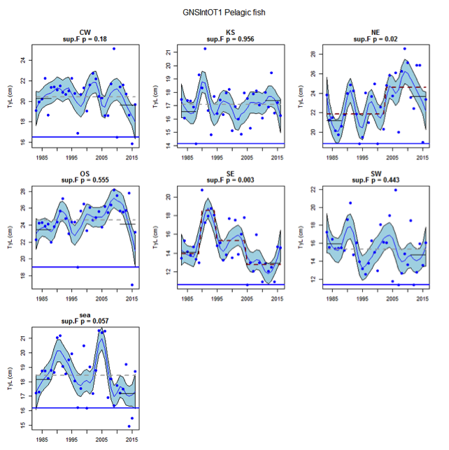
Figure t: Time series of Typical Length for each sub-division of the GNSIntOT1 survey (Pelagic fish)
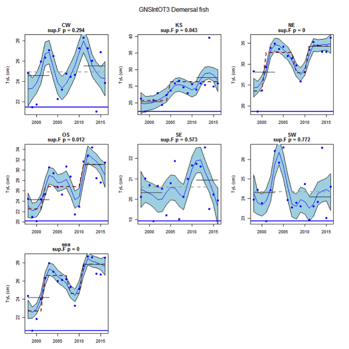
Figure u: Time series of Typical Length for each sub-division of the GNSIntOT3 survey (Demersal fish)
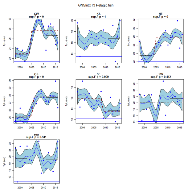
Figure v: Time series of Typical Length for each sub-division of the GNSIntOT3 survey (Pelagic fish)
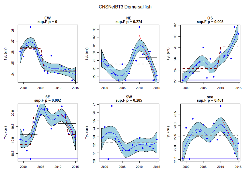
Figure w: Time series of Typical length for each sub-division of the GNSNetBT3 survey (Demersal fish)
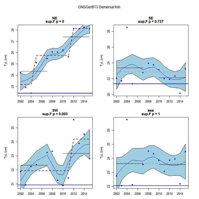
Figure x: Time series of Typical Length for each sub-division of the GNSGerBT3 survey (Demersal fish)
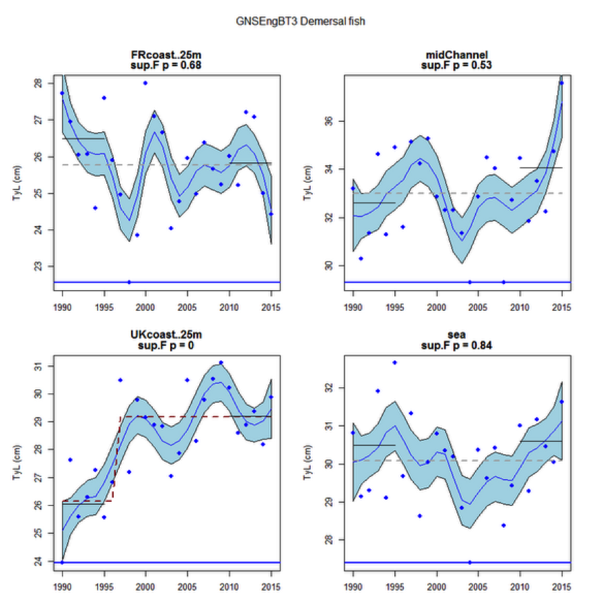
Figure y: Time series of Typical Length for each sub-division of the GNSEngBT3 survey (Demersal fish)
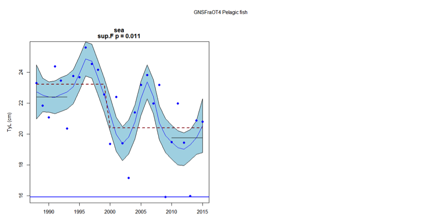
Figure z: Time series of Typical Length for each sub-division of the GNSFraOT4 survey (Pelagic fish)
Celtic Seas
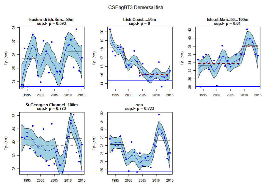
Figure aa: Time series of Typical Length for each sub-division of the CSEngBT3 survey (Demersal fish)
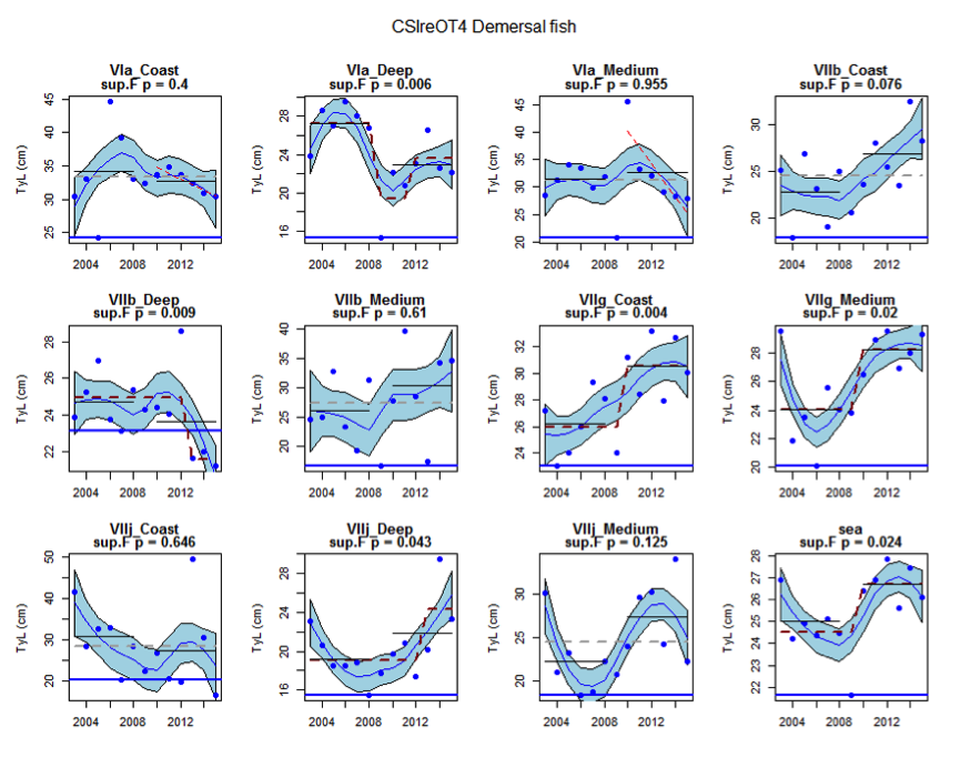
Figure ab: Time series of Typical Length for each sub-division of the CSIreOT4 survey (Demersal fish)
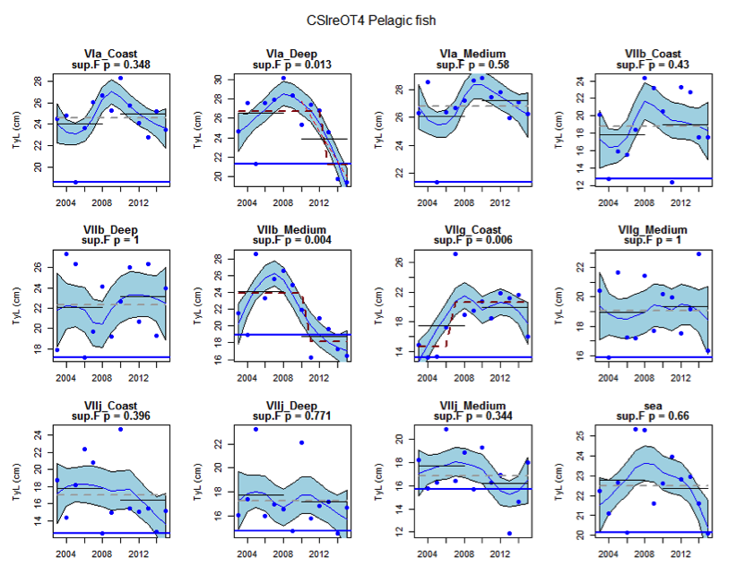
Figure ac: Time series of Typical Length for each sub-division of the CSIreOT4 survey (Pelagic fish)
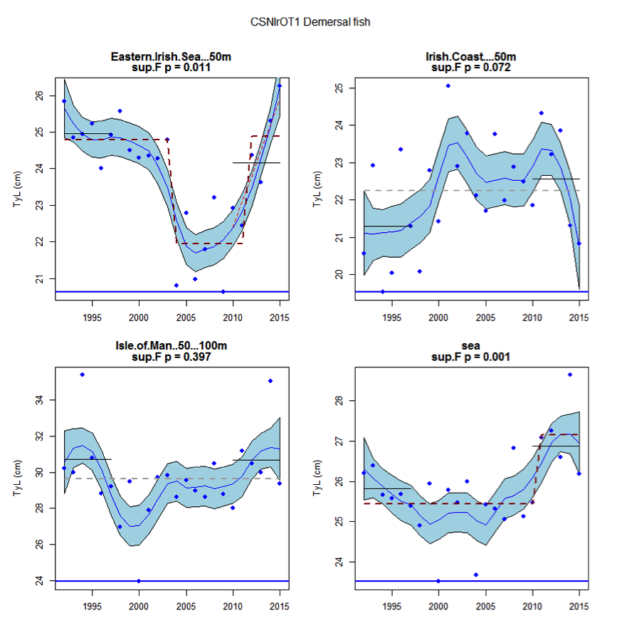
Figure ad: Time series of Typical Length for each sub-division of the CSNIrOT1 survey (Demersal fish)
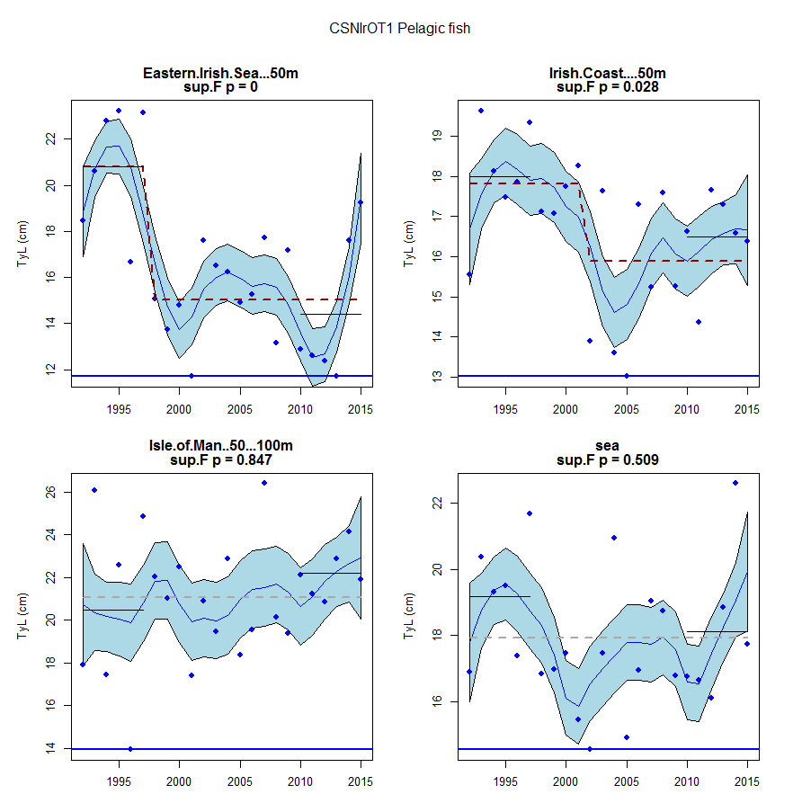
Figure ae: Time series of Typical Length for each sub-division of the CSNIrOT1 survey (Pelagic fish)
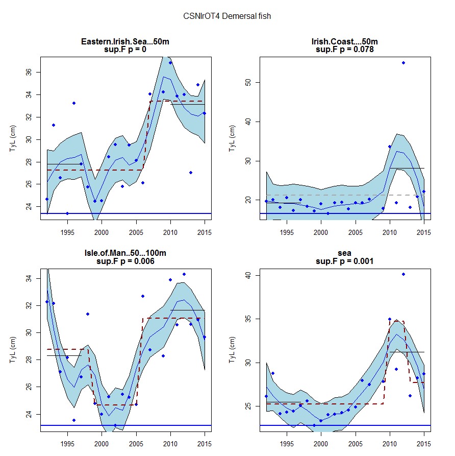
Figure af: Time series of Typical Length for each sub-division of the CSNIrOT4 survey (Demersal fish)
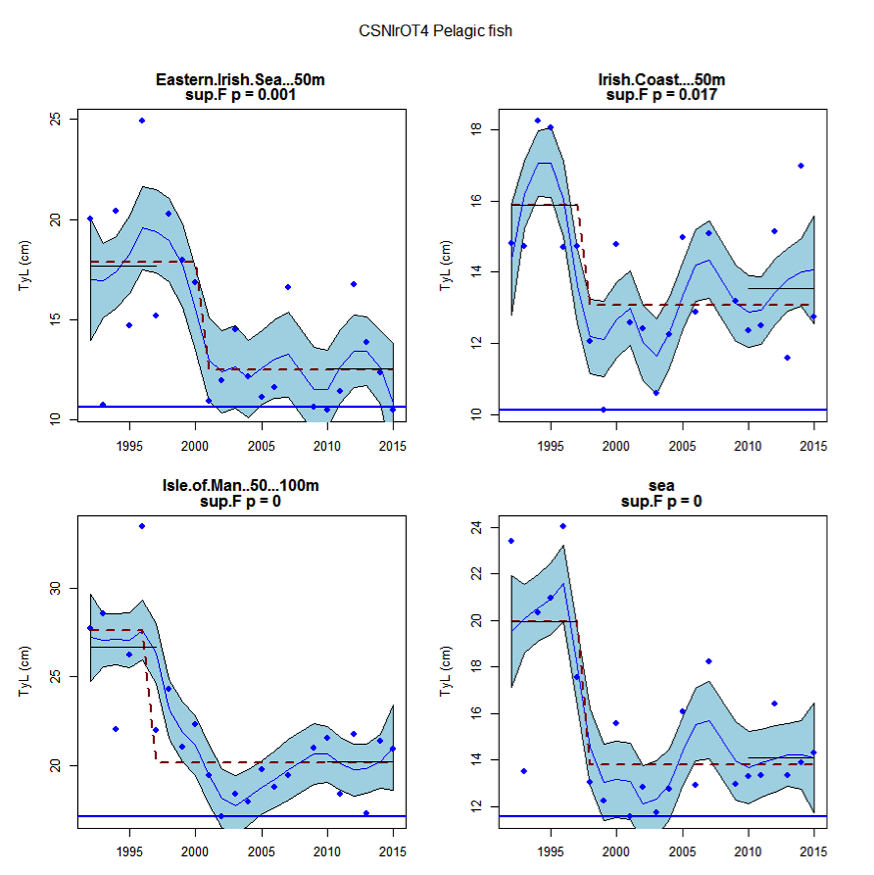
Figure ag: Time series of Typical Length for each sub-division of the CSNIrOT4 survey (Pelagic fish)
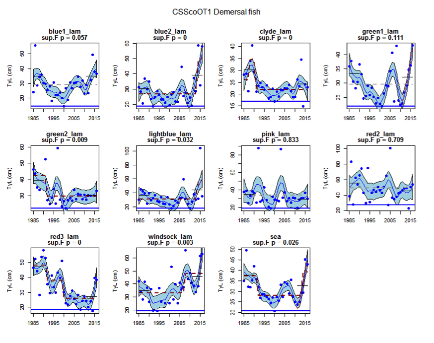
Figure ah: Time series of Typical Length for each sub-division of the CSScoOT1 survey (Demersal fish)
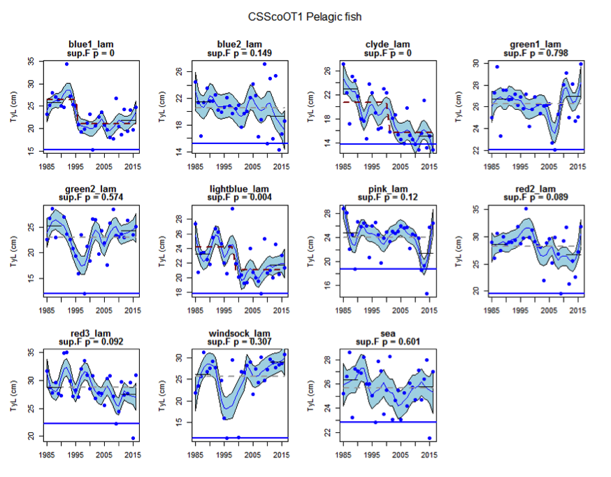
Figure ai: Time series of Typical Length for each sub-division of the CSScoOT1 survey (Pelagic fish)
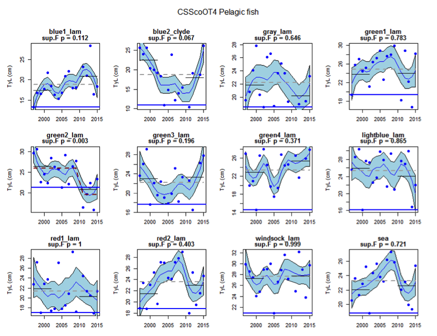
Figure aj: Time series of Typical Length for each sub-division of the CSScoOT4 survey (Pelagic fish)
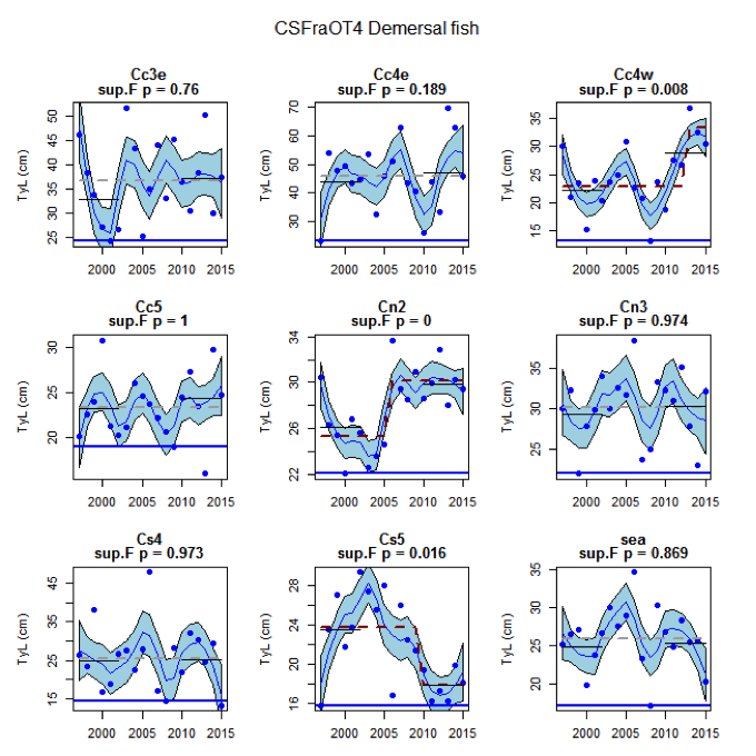
Figure ak: Time series of Typical Length for each sub-division of the CSFraOT4 survey (Demersal fish).
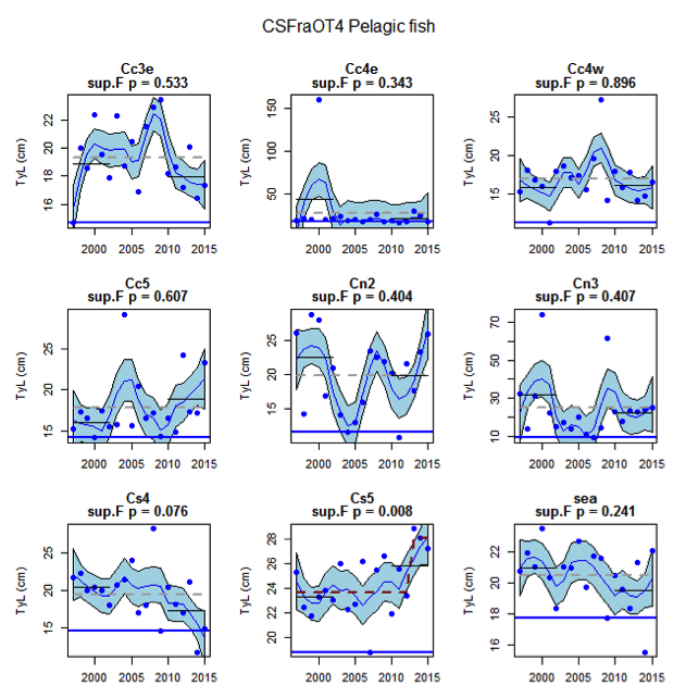
Figure al: Time series of Typical Length for each sub-division of the CSFraOT4 survey (Pelagic fish)
Bay of Biscay and the Iberian coast
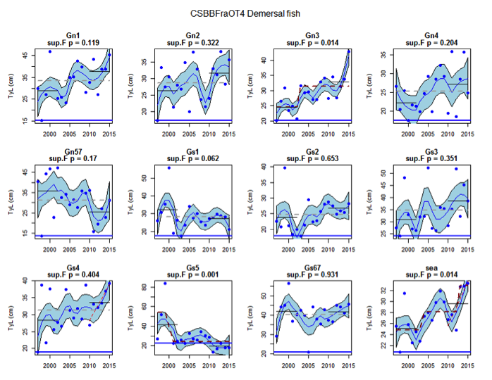
Figure am: Time series of Typical Length for the CSBBFraOT4 survey (Demersal fish)
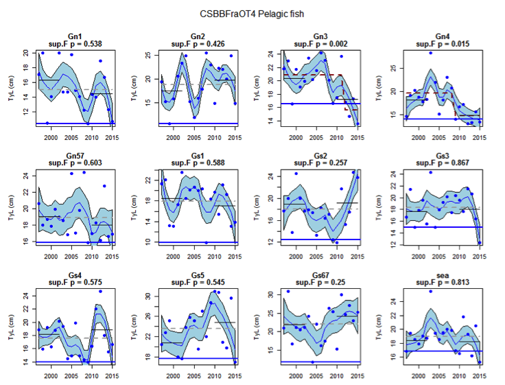
Figure an: Time series of Typical Length for each sub-division of the CSBBFraOT4 data (Pelagic fish)
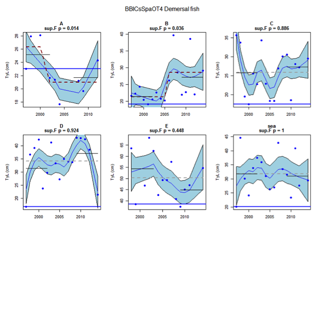
Figure ao: Time series of Typical Length for each sub-division of the BBIC(n)SpaOT4 data (Demersal fish)
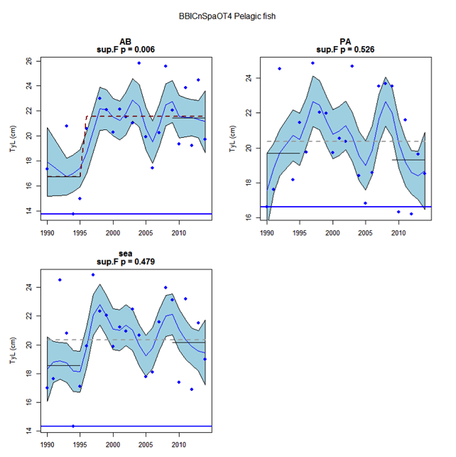
Figure ap: Time series of Typical Length for each sub-division of the BBIC(n)SpaOT4 survey (Pelagic fish)
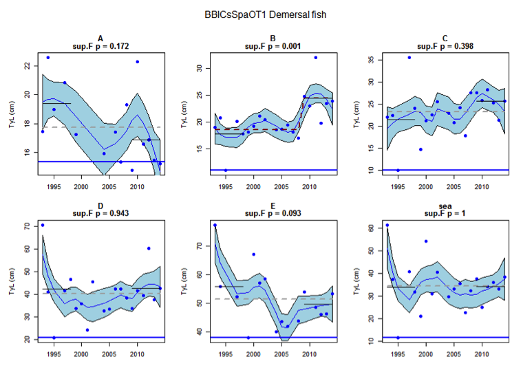
Figure aq: Time series of Typical Length for each sub-division of the BBIC(s)SpaOT1 survey (Demersal fish)
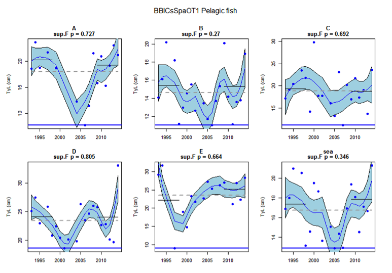
Figure ar: Time series of Typical Length for each sub-division of the BBIC(s)SpaOT1 survey (Pelagic fish)
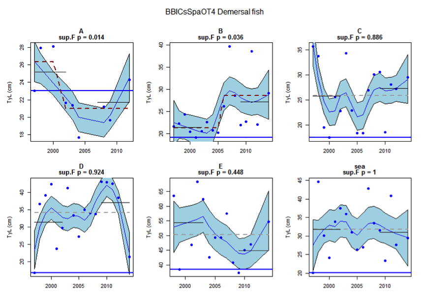
Figure as: Time series of Typical Length for each sub-division of the BBIC(s)SpaOT4 survey (Demersal fish)
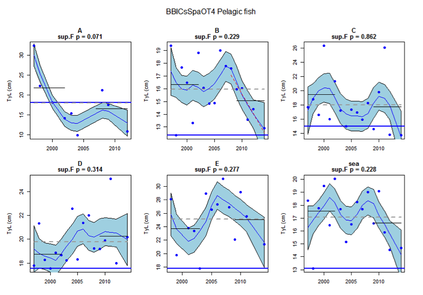
Figure at: Time series of Typical Length for each sub-division of the BBIC(s)SpaOT4 survey (Pelagic fish)
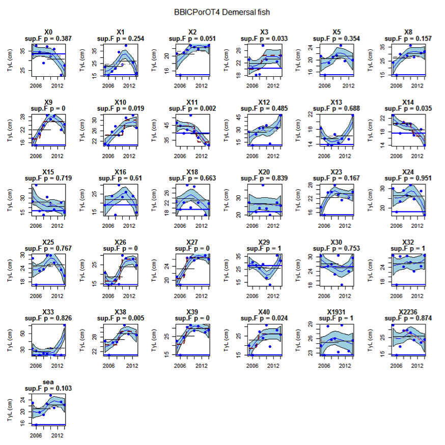
Figure au: Time series of Typical Length for each sub-division of the BBICPorOT4 survey (Demersal fish)
Wider Atlantic
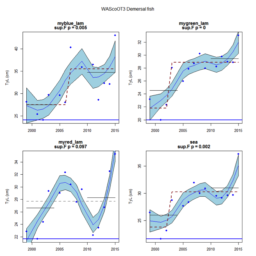
Figure av: Time series of Typical Length for each sub-division of the WAScoOT3 survey (Demersal fish)
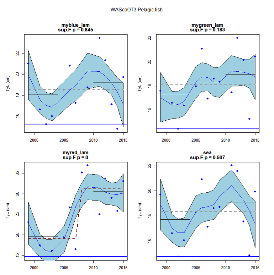
Figure aw: Time series of Typical Length for each sub-division of the WAScoOT3 survey (Pelagic fish)
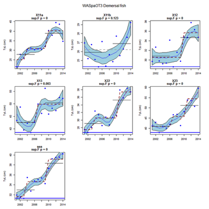
Figure ax: Time series of Typical Length for each sub-division of the WASpaOT3 survey (Demersal fish)
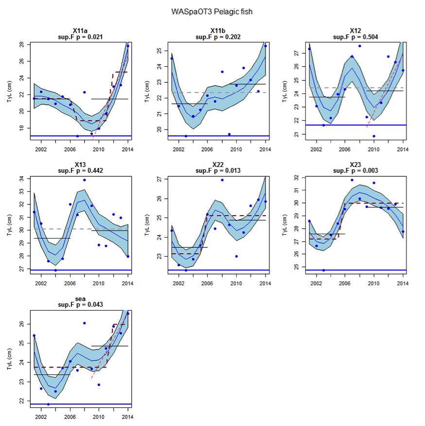
Figure ay: Time series of Typical Length for each sub-division of the WASpaOT3 survey (Pelagic fish)
Assessment of Confidence
The method has been developed specifically for this assessment. There is consensus within the scientific community regarding this methodology, however further methodological development is required therefore, it has been rated as moderate / low.
There are no significant data gaps and there is sufficient spatial coverage, confidence for data availability is rated as high.
Conclusion
Des diminutions à long terme de la longueur typique, entre les années 1980 et les années 2000, dans la mer du Nord au sens large et des années 1990 à 2005 dans les mers Celtiques, signifient que la détérioration de la structure des tailles des communautés halieutiques est telle que des poissons plus petits sont désormais dominants dans des communautés. On a relevé dans l’ensemble une augmentation dans l’Atlantique au large et le golfe de Gascogne et la côte ibérique, depuis 2010.
Cependant, l’indicateur des assemblages halieutiques démersaux demeure souvent à une valeur relativement basse, mais depuis 2010 un rétablissement de la longueur typique du poisson et des élasmobranches démersaux dans la mer du Nord au sens large et les mers Celtiques, semble se produire dans l’ensemble ou tout au moins dans quelques sous-divisions. L’assemblage halieutique pélagique ne révèle aucune modification à long terme dans la plus grande partie de la zone maritime OSPAR.
In the fish and elasmobranch community, Typical Length responds to changes in the dynamics of the size distribution across the full assemblage including both large and small fish, yet the indicator is still robust to outliers in the data. Typical Length can be directly compared across geographic regions and the indicator can be computed for pelagic or demersal species. The sub-divisional strata are a useful means to capture local patterns in the indicator for specific benthic and water column habitats and the often-local impacts of pressures.
Within the Greater North Sea there are clear sub-divisional differences, with demersal and pelagic assemblages in the northerly areas now recovering, while the southerly areas continue to decline. For the Celtic Seas, decreases in the demersal fish assemblage appear greatest at the shelf edge, while decreases in pelagic fish occur in coastal areas.
While fisheries may have contributed to this depletion, it is unclear whether rising sea temperatures have led to increases in small-bodied fish (i.e. young fish and / or small species). In the Bay of Biscay, where declines are seen in the size structure of pelagic fish, increases are evident in demersal fish.
In addition to the key surveys for each assessment region, additional survey information was assessed which generally confirmed the overall conclusions.
The increase in the typical length of demersal fish since 2010 in the Greater North Sea, evident in the International Bottom Trawl Survey (IBTS) quarter one (Q1) survey, was also shown in the quarter three (Q3) survey (GNSIntOT1 and GNSIntOT3), while the more spatially restricted groundfish surveys showed no significant change (GNSNetBT3, GNSGerBT3, GNSEngBT3). For pelagic fish, no change was evident in the two IBTS surveys in the Greater North Sea.
Within the Celtic Seas, increases in the typical length of demersal fish were evident to the west of Scotland in two surveys (CSScoOT1 since a low value in 2010 and CSScoOT4 since 2005), increases were evident in the Irish Sea in two surveys (CSNIrOT1 and CSNIrOT4 since 2010) with no change in a third (CSEngBT3), to the south and west of Ireland increases were evident in one survey (CSIreOT4 since 2010). The pelagic fish generally showed no significant changes in typical length, with the exception of a decrease in the Irish Sea in one survey (CSNIrOT4 in 1998).
For the Bay of Biscay and Iberian coast, the typical length of demersal fish increased in two of the five available surveys (CSBBFraOT4 since 2004 and BBICnSpaOT4 since 1998) and no overall changes in the typical length of pelagic fish were detected.
An overall increase since 2002 in the typical length of demersal fish in the Wider Atlantic were significant in both assessed surveys (WAScoOT3 and WASpaOT3). No change in the typical length of pelagic fish was evident in WAScoOT3 but an increase from 2012 was evident in the WASpaOT3 survey.
Lacunes des connaissances
Il y a lieu d’entreprendre des travaux supplémentaires pour évaluer des lignes de base et des valeurs d’évaluation adéquates pour cet indicateur. En effet il est fort probable que toute ligne de base historique pour les communautés halieutiques et d’élasmobranches représente un état ayant subi des impacts. Il faudra identifier des valeurs d’évaluation, de préférence grâce à une modélisation à espèces multiples.
The setting of assessment values for this indicator should consider their relation to the European Union’s Common Fisheries Policy targets aiming at Maximum Sustainable Yield and in relation to other fish community indicators.
Until more comprehensive investigations are complete, the minimum observed typical length in the available time series can be considered as a precautionary limit for the indicator. If indicator scores are at a minimum observed state, a positive (increasing) trend should be evident to avoid falling below the limit.
While reductions in fishing pressure in recent years appear to be driving improvements in the size structure of the demersal fish community in some areas, it should not be forgotten that the OSPAR Maritime Area has also warmed significantly recently (IPCC, 2014). These prevailing conditions may mean species composition is changing. Since Lusitanian (warm-water southern) species tend to be smaller bodied than boreal (cold-water northern) species, the size-structure may require longer than expected to recover to its historic values, if possible.
Barnes et al. (2010) Global patterns in predator–prey size relationships reveal size dependency of trophic transfer efficiency Ecology, 91(1), 222–232
Boudreau P. R., L. M. Dickie (1992) Biomass Spectra of Aquatic Ecosystems in Relation to Fisheries Yield. Canadian Journal of Fisheries and Aquatic Sciences, 1992, 49:1528-1538, 10.1139/f92-169
Commission Regulation (EC) No 665/2008 of 14 July 2008 laying down detailed rules for the application of Council Regulation (EC) No 199/2008 concerning the establishment of a Community framework for the collection, management and use of data in the fisheries sector and support for scientific advice regarding the Common Fisheries Policy, http://data.europa.eu/eli/reg/2008/665/oj
Daufresne M., Lengfellner K. and Sommer U. (2009) Global warming benefits the small in aquatic ecosystems PNAS 106 (31) 12788-12793, doi:10.1073/pnas.0902080106
Fraser, H. M., Greenstreet, S. P. R., and Piet, G. J. 2007. Taking account of catchability in groundfish survey trawls: implications for estimating demersal fish biomass. ICES Journal of Marine Science, 64: 1800–1819
Fung, T., Farnsworth, K. D., Shephard, S., Reid, D. G., and Rossberg, A. G. 2013. Why the size structure of marine communities can require decades to recover from fishing. Marine Ecology Progress Series, 484, 155—171. doi:10.3354/meps10305.
Gibert JP, DeLong JP. 2014 Temperature alters food web body-size structure. Biol. Lett. 10: 20140473. http://dx.doi.org/10.1098/rsbl.2014.0473
ICES, 2014a - Report of the Working Group on the Ecosystem Effects of Fishing Activities (WGECO). ICES Document CM 2014/ACOM:26, Copenhagen, Section 3.4.3 (http://tinyurl.com/p8vwu7d)
ICES. 2014b. Interim Report of the Working Group on Multispecies Assessment Methods (WGSAM), 20–24 October 2014, London, UK. ICES CM 2014/SSGSUE:11
IPCC, 2014: Climate Change 2014: Synthesis Report. Contribution of Working Groups I, II and III to the Fifth Assessment Report of the Intergovernmental Panel on Climate Change [Core Writing Team, R.K. Pachauri and L.A. Meyer (eds.)]. IPCC, Geneva, Switzerland, 151 pp.
Jennings, S., Oliveira, J. A. A. D. and Warr, K. J. (2007), Measurement of body size and abundance in tests of macroecological and food web theory. Journal of Animal Ecology, 76: 72–82. doi:10.1111/j.1365-2656.2006.01180.x
Kerr, S. R. & Dickie, L. M. 2001. The biomass spectrum: a predator– prey theory of aquatic production. New York, NY:Columbia University Press.
Lynam C.P. and A.G. Rossberg. (2017) New univariate characterization of fish community size structure improves precision beyound the Large Fish Indicator. Available: at arXiv:1707.06569
Probst WN, Stelzenmüller V (2015) A benchmarking and assessment framework to operationalise ecological indicators based on time series analysis. Ecological Indicators 55: 94-106, doi:10.1016/j.ecolind.2015.02.035
Reum, J. C. P., Jennings, S. and Hunsicker, M. E. (2015), Implications of scaled δ15N fractionation for community predator–prey body mass ratio estimates in size-structured food webs. J Anim Ecol, 84: 1618–1627. doi:10.1111/1365-2656.12405
Riede, J. O., Brose, U., Ebenman, B., Jacob, U., Thompson, R., Townsend, C. R. and Jonsson, T. (2011), Stepping in Elton’s footprints: a general scaling model for body masses and trophic levels across ecosystems. Ecology Letters, 14: 169–178. doi:10.1111/j.1461-0248.2010.01568.x
Rossberg, A. G., Ishii, R., Amemiya, T. and Itoh, K. (2008). The top-down mechanism for body-mass–abundance scaling. Ecology, 89: 567–580. doi:10.1890/07-0124.1
Rossberg, A. G. (2012). A complete analytic theory for structure and dynamics of populations and communities spanning wide ranges in body size. Advances in Ecological Research, 46, 429-522
Shephard, S., Fung, T., Houle, J. E., Farnsworth, K. D., Reid, D. G., and Rossberg, A. G. 2012. Size-selective fishing drives species composition in the Celtic Sea. ICES Journal of Marine Science, 69: 223–234
Walker, N. D., Maxwell, D. L., Le Quesne, W. J. F., and Jennings, S. (2017) Estimating efficiency of survey and commercial trawl gears from comparisons of catch-ratios. ICES Journal of Marine Science, doi:10.1093/icesjms/fsw250