

Composition et répartition spatiale des déchets sur le sol marin
D10 - Déchets marins
D10.1 - Caractéristiques des déchets présents dans l’environnement marin et côtier
Message clé:
Les déchets sont très répandus sur le sol marin dans l’ensemble de la zone évaluée, les déchets plastiques étant prédominants. Les quantités de déchets sont plus importantes dans la partie orientale du golfe de Gascogne, les mers Celtiques méridionales et la Manche que dans la mer du Nord au sens large septentrionale et les mers Celtiques septentrionales.
Zone Évaluée
Récapitulatif Imprimable
Contexte
Les déchets marins présentent un problème à l’échelle planétaire, des quantités croissantes étant notifiées ces dernières décennies. L’abondance des déchets sur le sol marin est influencée par des apports anthropiques, notamment les déchets transportés par les fleuves et les courants océaniques qui peuvent les redistribuer sur de grandes distances. Les déchets marins sont donc un problème transfrontalier.
Des animaux marins peuvent ingérer, ou s’emmêler dans, des déchets (par exemple des engins de pêche abandonnés, des bandes de cerclage) sur le sol marin ou à proximité. Cette situation pourrait entraîner la mort ou des blessures, par exemple en suffoquant ou en laissant mourir de faim des animaux. Les déchets plastiques sont des vecteurs potentiels de contaminants et peuvent également causer une abrasion ou un étouffement du sol marin. Ceci pourrait avoir un impact sur les habitats benthiques fragiles en réduisant la photosynthèse et en empêchant le mouvement des animaux, des gaz et des nutriments. Les déchets marins peuvent également jouer le rôle de vecteur pour des espèces envahissantes, transportant des organismes non indigènes dans de nouvelles zones ou ils peuvent faire concurrence aux organismes indigènes ou les utiliser comme proies.
On a étudié les déchets sur le sol marin aussi bien dans les eaux côtières qu’au large. La présence de grandes quantités de déchets plastiques sur le plateau continental européen a été notifiée. Les études du chalutage benthique sont une méthode pratique de surveiller les déchets sur le sol marin (sur le plateau continental) car elles sont déjà utilisées pour les évaluations des stocks halieutiques, couvrent une grande surface du sol marin et recueillent une quantité suffisante de déchets pour les analyses.
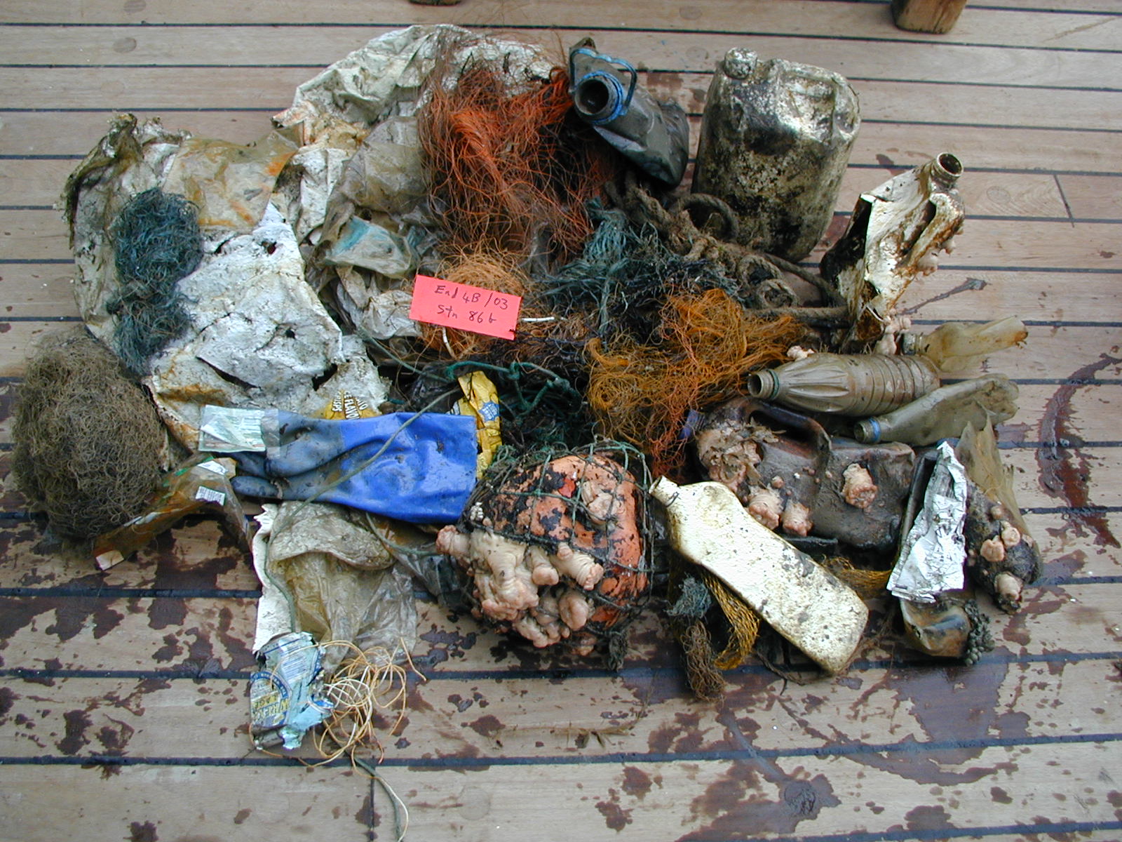
Image: Capture accessoires de déchets marins à bord du navire de recherche Endeavour ©J. Thain
Litter on the seafloor has been studied in both coastal and deep sea waters using techniques that include snorkelling, SCUBA diving, trawl surveys, sonar and the use of manned and unmanned submersibles (Spengler and Costa, 2008; Miyake et al., 2011 Watters et al., 2010; Bergmann and Klages, 2012; Galgani et al., 2013; Schlining et al., 2013). The presence of large amounts of plastic litter has been reported in European continental shelf seas (Galgani et al., 2000; Pham et al., 2014), including in the Baltic Sea, the North Sea, the Celtic Sea, the Bay of Biscay (Galgani et al., 1995a), the Mediterranean Sea (Galgani et al., 1995b, 1996; Galil et al., 1995; Stefatos et al., 1999), the Adriatic Sea (Bingel et al., 1987) and the Black Sea (Loakeimidis et al., 2014). On continental shelves, trawl surveys are a practical way to monitor seafloor litter because they are already used for fish stock assessments, cover a wide area of the seafloor and collect a sufficient quantity of litter for analysis.
Benthic trawls (Figure a) are designed to capture marine biota on or near the seafloor over a range of different seabed types. As a result, some trawl designs will plough through the seafloor while others roll over the seafloor. This interaction with the seafloor together with the mesh size will influence the amounts of litter captured during a survey.
As the trawl passes across the seafloor, litter is ‘kicked up’ into the water. Because plastics are prone to drifting they are more likely to remain suspended long enough be retained in the cod-end (see Figure a). In contrast, metals, glass and ceramics and other heavier materials are more likely to drop out through the mesh before reaching the cod-end. As a result, different litter types have different catchabilities and so are differently represented in the catch (Moriarty et al., 2016). However, because these differences in catchability are relatively constant and should show little change from survey to survey, the survey results can still be compared. Furthermore, plastics (which have the highest catchability) are of greatest concern in terms of harm.
Thus, although the sampled quantities are ‘relative’ rather than absolute numbers, they can be used to compare regions sampled with similar gear. The number of stations monitored will determine the confidence that can be applied to the assessments and define the time (number of years of survey data) that will be needed to obtain an acceptable confidence in the assessment.
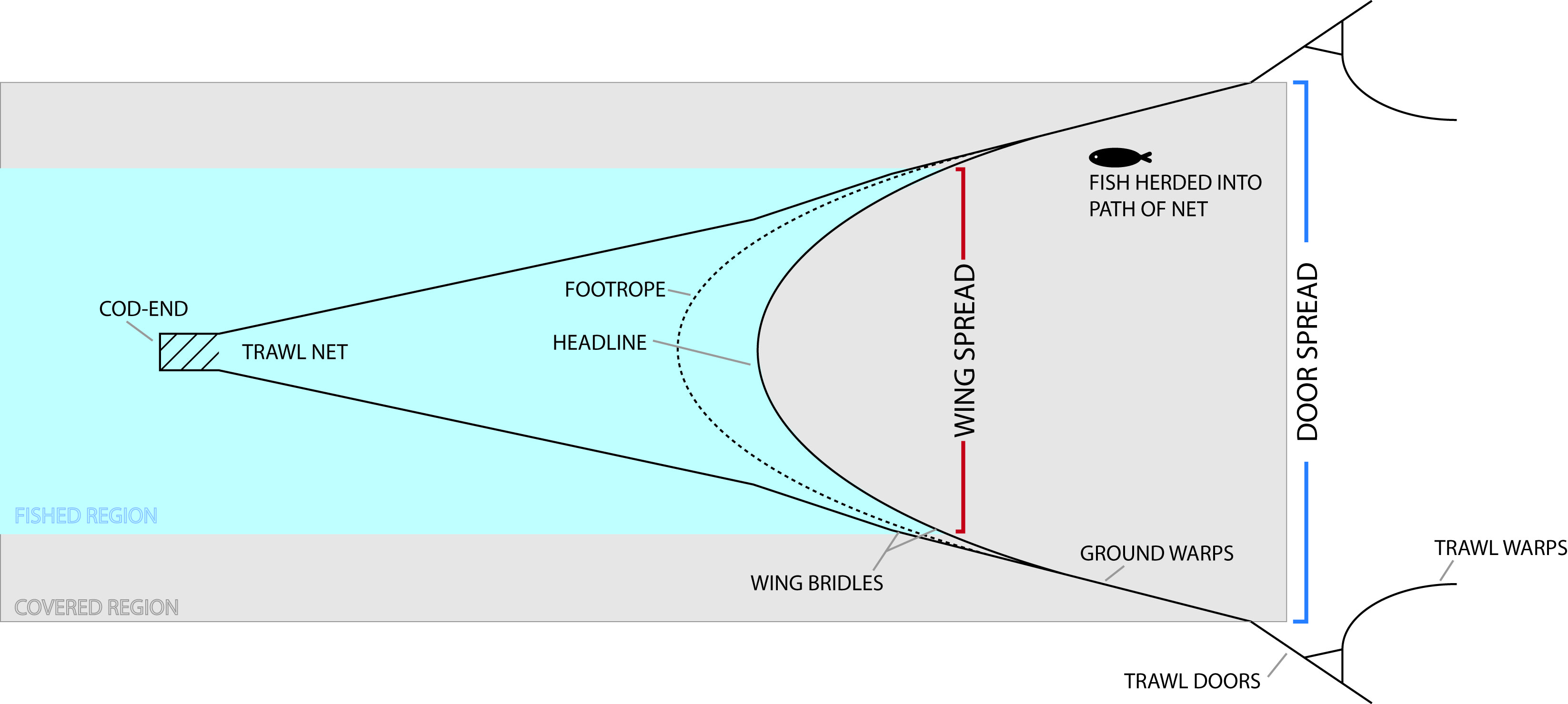
Figure a: The active region of a trawl. Door spread is shown in blue and wing spread is shown in red (Adapted from Carrothers, 1980).
As part of the implementation of the OSPAR North-East Atlantic Environment Strategy, OSPAR has adopted a common indicator on seafloor litter in response to the European Union (EU) Marine Strategy Framework Directive (MSFD) Criterion 10.1.2: Trends in the amount of litter in the water column (including floating at the surface) and deposited on the seafloor, including analysis of its composition, spatial distribution and, where possible, source.
In order to assess the indicator, it was necessary to collect litter data that has been gathered by existing fisheries trawl surveys. OSPAR Contracting Parties agreed to submit litter data to the International Council for the Exploration of the Sea (ICES), which has developed databases to hold these data. Seafloor litter monitoring data, generated through existing fisheries trawl surveys, was requested for 2012 onwards.
The majority of the seafloor litter data originated from surveys organised by the International Bottom Trawl Survey Working Group (IBTSWG), which coordinates fishery-independent multispecies bottom trawl surveys within the ICES area. The main objective of the surveys is the long-term monitoring of demersal fish, to provide ICES and science groups with consistent and standardised data for commercial fish stock assessments. Marine litter data is collected as part of these fish stock surveys and thus follows a sampling strategy as outlined by IBTSWG.
Ideally, the trawl wing spread (i.e. the width of the opening of the net, outlined in red in Figure a) would be used for calculating litter counts as it provides a more accurate calculation of litter items per km2. However this measurement is not always available so the door spread (i.e. the distance between the trawl doors, outlined in blue in Figure a) must be used instead and a conversion factor applied to the data.
Details regarding the data used
Litter data collected during fisheries trawl surveys are submitted directly to the Database of Trawl Surveys (DATRAS). The format, including field descriptions can be found on the ICES website, dataset name ‘Litter data from DATRAS surveys’, reference document ‘Litter_Format_DATRAS’, more information can also be found in the Guidance on Monitoring of Marine Litter in European Seas, (Galgani et al, 2013). The data include seafloor litter data from fisheries trawl surveys for the period 2012–2014 undertaken in the OSPAR Maritime Area. The data will be available through the ICES Data Portal on the ICES website http://ecosystemdata.ices.dk/.
Because this is the first OSPAR-wide seafloor litter assessment of this type there were some initial data issues. Due to time constraints some pragmatic decisions were taken concerning the management and processing of the data :
- Some rows in the original data file that seemed largely to contain missing values were deleted.
- There were 177 values of -9 in the ‘items’ field, these were recoded as zero.
- Data from 2011 (54 values) and from 2015 (1023 values) were excluded. Only data for 2012–2014 were used.
- Only Grande Ouverture Verticale (GOV) trawl values were used for the Greater North Sea, the Celtic Seas and the Eastern Bay of Biscay so that the gear type was comparable across those regions.
- Only BAK trawl values were used for the north-western Iberian Coast and the Gulf of Cadiz so that the gear type was comparable across those regions.
- The data format was not in an appropriate form for easy analysis. For every haul, there was a new line for each litter item found. The data format was modified and a data file was produced where every line is a haul and where there are columns for the number of litter items found in each haul as well as many explanatory variables about the haul.
- It is better to use wingspan rather than door spread to summarise the cross-sectional area. However, there was more complete information for door spread (140 missing entries) than wing spread (802 missing entries). The following was used to define haul ‘area’: area = 1000 000 × litter / (door spread distance) km2. The “1000 000” is because distance is measured in metres. This value may not give the best measurement of haul area but it does provide a measurement of relative area that is comparable across regions and years.
- To more accurately predict the number of items per km2 the mean of the door / wing ratios (4.18) was used as an approximate conversion factor.
- If a haul contained no litter items, then a code (RECO-LT) was given to say this and all litter counts for that trawl were set to zero. There are two lines with this code for which the number of litter items in the original data set was 1. These were set to 0.
- There were two ways of coding the litter types: the older format (C-TS) and the revised (C-TS-REV) format. The vast majority of entries in the original file used the old method (6614) as opposed to the new method (358). Having two entry methods increases the difficulty of getting the data into an appropriate form for analysis.
Presentation of results
The figures presented in the results show spatially smoothed predictions of litter type at points on a grid. The grid used to produce the figures is 200 (longitude) by 127 (latitude) of equally spaced points. Grid points that are more than 20 km from a monitoring station are not used. The plots were smoothed using a Generalised Linear Model (Wood, 2006) with longitude and latitude as the explanatory variables. The counts were modelled using a negative binomial family and the litter per km2 values were ln(x+1) transformed in an attempt to get them approximately Gaussian (with limited success). For the litter per km2 plot, the smoothed values were back-transformed using an exponential minus one transformation. The plots are thus approximately median levels on the original scale. For the power studies the trend.power function in the R library emon (Barry and Maxwell et al., 2015) was used. The Manly approach (Manly et al., 2007), a nonparametric randomisation test, was used to make comparisons between surveys and OSPAR areas. For total litter and for plastic, 95% bootstrap confidence intervals are also given using the percentile method (see Table c and Table d) (Manly et al., 2007).
Résultats
La répartition et l’abondance des déchets marins sur le sol marin de la Zone maritime OSPAR ont été étudiées en se fondant sur les données recueillies par les études du chalutage de sept Parties contractantes (Figure 1). Les chaluts benthiques sont conçus pour capturer des organismes marins sur divers types de sol marin ou à proximité. Certains chaluts sont donc conçus de telle sorte qu’ils labourent le sol marin alors que d’autres roulent sur le sol marin. La quantité de déchets capturés au cours d’une étude dépend du type d’interaction avec le sol marin et du maillage des filets. Les quantités échantillonnées ne sont donc pas des quantités absolues mais des quantités « relatives ». Elles permettent cependant des comparaisons entre des régions échantillonnées avec des engins semblables. Le nombre de stations surveillées détermine la confiance pouvant être appliquée aux évaluations et définit la durée (nombre d’années de données) nécessaire pour obtenir un niveau de confiance acceptable.
La répartition des déchets, en particulier plastiques, est très répandue sur le sol marin de la mer du Nord au sens large, la mer Celtique, le golfe de Gascogne, la côte ibérique et le golfe de Cadix. L’évaluation se focalise principalement sur la mer du Nord au sens large, les mers Celtiques et la partie orientale du golfe de Gascogne (la côte ibérique et le golfe de Cadix sont exclus) l’échantillonnage ayant été réalisé avec un chalut à grande ouverture verticale (GOV). L’abondance des déchets individuels (nombre d’objets par km2) sur le sol marin de cette zone augmente du nord au sud (Figure 2). En 2014, de tous les déchets marins enregistrés, le pourcentage des objets en plastique s’élevait à 68% pour la mer du Nord au sens large, 58% pour la mer Celtique et 98% pour la partie orientale du golfe de Gascogne. Presque tous les chaluts dans la partie orientale du golfe de Gascogne possédaient au moins un objet en plastique; cette zone possède également les niveaux les plus élevés de déchets enregistrés au sein de la zone évaluée.

Figure 1: Stations utilisées pour évaluer les déchets sur le sol marin.
Endroits d’échouage des déchets en mer du Nord au sens large, dans les mers Celtiques et la partie orientale du golfe de Gascogne (GOV; orange) et la côte ibérique et le golfe de Cadix (BAK; mauve)
Il n’a pas été possible de faire une comparaison directe entre les résultats portant sur la mer du Nord au sens large et les mers Celtiques, qui utilisent un chalut GOV, et ceux de l’évaluation de la côte ibérique et du golfe de Cadix dont l’échantillonnage est réalisé avec un chalut à panneaux BAK (voir la Figure 1). Il n’a pas été possible de créer une carte de l’abondance relative des déchets pour la côte ibérique et le golfe de Cadix, semblable à la Figure 2 car les échantillons étaient groupés près de la côte, étant donné la topographie.
Le degré de confiance dans la méthodologie est modéré et celui des données est faible à modéré.
Figure 2: Nombre relatif d’objets par km2 de sol marin dans l’ensemble de la mer du Nord au sens large, des mers Celtiques et de la partie orientale du golfe de Gascogne, basé sur le nombre d’objets pris accidentellement dans les chaluts.
Data analysis
The distribution and abundance of marine litter on the seafloor in the OSPAR Maritime Area was investigated on the basis of data generated by trawl surveys from seven countries (Denmark, France, Germany, the Netherlands, Spain, Sweden and the United Kingdom). Two separate assessments were made: one using Grande Ouverture Verticale (GOV) trawl data and one for data collected by BAK trawl (Figure 1). The GOV assessment was based on 670 hauls in 2012, 790 hauls in 2013 and 794 hauls in 2014. These were undertaken across three OSPAR regions: the Greater North Sea, the Celtic Seas and the Bay of Biscay. For the Spanish BAK assessment there were 182 hauls in 2012, 197 hauls in 2013 and 160 hauls in 2014 across two sub-regions: the Iberian Coast and the Gulf of Cadiz. For GOV trawls, the numbers of hauls by region and year are summarised in Table a.
Widespread distribution of litter items, especially plastics, was discovered on the seafloor of the Greater North Sea, the Celtic Seas, the Eastern Bay of Biscay, the Iberian Coast and the Gulf of Cadiz. Table b shows the proportion of all litter items that are plastic by year and region for the GOV data. The Celtic Seas have a particularly high proportion of plastic items. Ideally, the number of items found would be standardised to the area of the haul. This is effectively the distance of the haul multiplied by the cross-sectional area of the net (Figure a). Although it would be better to use wing spread to determine the cross-sectional area of the net, due to missing data values this was not possible and door spread was used instead, with the mean of the door / wing ratios (4.18) used as an approximate conversion factor to generate wing spread values. Table c, Table d and Table e present data showing how the litter items collected in the GOV trawls changed over the three years of the study for each region. Although there appear be differences between years, at least five years of data are required to be able to make confident statements regarding trends.
| Celtic Seas | Greater North Sea | Eastern Bay of Biscay | |
|---|---|---|---|
| 2012 | 254 | 358 | 58 |
| 2013 | 225 | 496 | 69 |
| 2014 | 210 | 503 | 81 |
| Celtic Seas | Greater North Sea | Eastern Bay of Biscay | |
|---|---|---|---|
| 2012 | 0.90 | 0.62 | 0.66 |
| 2013 | 0.93 | 0.75 | 0.76 |
| 2014 | 0.95 | 0.85 | 0.87 |
| Region | Celtic Seas | Greater North Sea | Eastern Bay of Biscay | ||||||
|---|---|---|---|---|---|---|---|---|---|
| Year | 2012 | 2013 | 2014 | 2012 | 2013 | 2014 | 2012 | 2013 | 2014 |
| Total | 13.794 (10.868, 16.72) | 48.07 (30.514, 71.06) | 48.906 (35.948, 63.954) | 28.842 (25.08, 32.604) | 30.932 (27.588, 34.276) | 38.038 (34.276, 41.8) | 96.14 (78.166, 115.786) | 230.736 (149.644, 325.622) | |
| Plastic | 11.704 (9.196, 14.212) | 44.726 (28.006, 66.044) | 46.398 (33.022, 62.7) | 17.974 (15.466, 20.064) | 22.99 (20.9, 25.498) | 32.186 (28.842, 35.948) | 75.658 (62.7, 88.198) | 203.566 (129.58, 299.288) | |
| Metal | 0.29 | 0.88 | 0.79 | 1.30 | 0.84 | 0.96 | - | 1.46 | 0.96 |
| Rubber | 0.17 | 0.79 | 0.38 | 1.13 | 1.05 | 1.21 | - | 1.05 | 1.55 |
| Glass | 0 | 0.04 | 0 | 0.42 | 0.84 | 0.38 | - | 2.59 | 0.67 |
| Natural | 0.67 | 1.17 | 0.59 | 6.06 | 3.51 | 2.13 | - | 13.38 | 16.72 |
| Misc | 0.84 | 0.50 | 0.54 | 2.09 | 1.46 | 1.21 | - | 2.09 | 7.11 |
| Celtic Seas | Greater North Sea | Eastern Bay of Biscay | |||||||
|---|---|---|---|---|---|---|---|---|---|
| 2012 | 2013 | 2014 | 2012 | 2013 | 2014 | 2012 | 2013 | 2014 | |
| Total | 7.9 (6.3, 9.6) | 13.0 (9.2, 18.8) | 14.21 (10.0, 18.0) | 6.7 (5.9, 7.5) | 7.5 (6.7, 8.8) | 9.6 (8.4, 10.5) | 28.8 (18.8, 44.7) | 31.4 (19.2, 28.8) | 57.7 (35.1, 66.9) |
| Plastic | 7.1 (5.9, 8.80 | 12.1 (7.9, 17.1) | 13.8 (7.9, 18.0) | 4.18 (3.8, 4.6) | 5.9 (5.4, 6.3) | 7.9 (7.1, 9.2) | 19.2 (15.5, 22.6) | 23.8 (19.2, 28.8) | 50.1 (34.4, 66.9) |
| Metal | 0.17 | 0.25 | 0.25 | 0.29 | 0.21 | 0.25 | 0.42 | 0.42 | 0.29 |
| Rubber | 0.04 | 0.21 | 0.13 | 0.25 | 0.25 | 0.29 | 0.08 | 0.38 | 0.42 |
| Glass | 0.04 | 0.00 | 0 | 0.13 | 0.17 | 0.08 | 0.21 | 0.96 | 0.21 |
| Natural | 0.33 | 0.33 | 0.17 | 1.42 | 0.88 | 0.59 | 0.88 | 4.84 | 4.64 |
| Misc | 0.21 | 0.13 | 0.17 | 0.46 | 0.38 | 0.29 | 8.28 | 0.79 | 1.92 |
| Celtic Seas | Greater North Sea | Eastern Biscay of Biscay | |||||||
|---|---|---|---|---|---|---|---|---|---|
| 2012 | 2013 | 2014 | 2012 | 2013 | 2014 | 2012 | 2013 | 2014 | |
| Total | 61 (54,67) | 59 (52,65) | 64 (58,70) | 64 (59,69) | 70 (66,74) | 71 (67,75) | 95 (88,1) | 100 (100,1) | 100 (100,1) |
| Plastic | 59 (53,65) | 56 (49,62) | 58 (51,64) | 55 (50,61) | 64 (60,68) | 68 (63,72) | 93 (86,98) | 97 (93,1) | 98 (94,1) |
| Metal | 4 | 5 | 5 | 7 | 5 | 6 | 10 | 9 | 7 |
| Rubber | 1 | 5 | 2 | 6 | 6 | 7 | 2 | 7 | 9 |
| Glass | 0 | 0 | 0 | 2 | 3 | 2 | 5 | 4 | 1 |
| Natural | 4 | 6 | 4 | 16 | 13 | 10 | 3 | 23 | 31 |
| Misc | 5 | 2 | 3 | 10 | 7 | 6 | 16 | 14 | 25 |
There is wide variation in terms of abundance, with higher amounts of litter and plastic per km2 in the Eastern Bay of Biscay. Figure 2 and Table c show the number of litter items per km2 for all GOV trawls. The Eastern Bay of Biscay is the area of most litter, particularly for plastic items. Figure c and Table d and give similar information, except that the figures are based on the number of items caught per haul only, Figure d shows also show just the total number of plastic items caught per haul. Not weighting by haul area does not have a major effect on the assessment outcomes because most hauls are of similar area. Table e gives the percentage of hauls in which each of the litter types was found at least once. The results for the Eastern Bay of Biscay are notable with nearly all of the trawls in the Eastern Bay of Biscay contained at least one plastic item (Figure b).
Figure b: The modelled probability that a haul will contain plastic (from 1 where you will always find plastic to 0 where you will never find plastic)
Figure c: Total counts of litter items caught per trawl in the Greater North Sea, Celtic Sea and the Eastern Bay of Biscay
Figure d: Total counts of plastic items caught in trawls in Greater North Sea, Celtic Sea and the Eastern Bay of Biscay
The statistical power (the likelihood that a study will detect an effect when there is an effect there to be detected) was calculated with total litter counts for each of the three areas: Celtic Seas, Greater North Sea and the eastern Bay of Biscay. The sample size for each year was fixed at the following values (which correspond with the number of stations surveyed each year), 225 stations in the Celtic Seas, 500 stations in the Greater North Sea and 75 stations in the eastern Bay of Biscay. A starting mean for each region corresponding to the observed 2012 mean was assumed. The statistical power was then calculated for 10%, 20% and 30% increases over 5, 10, 15, 20, 25 and 30 years. A negative binomial distribution was assumed for the distribution of numbers of items per haul. The results are shown in Figure e. The Greater North Sea is the only region where there are sufficient stations to detect 20% or 30% changes with a statistical power of more than 90% (Figure e).
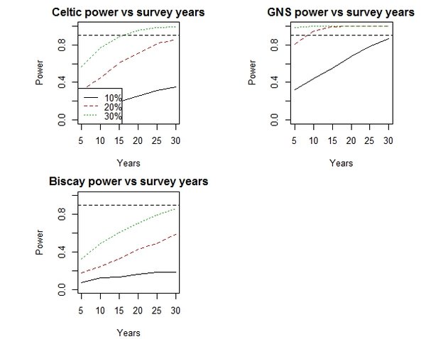
Figure e: Power plots for total litter items per haul for the Greater North Sea, Celtic Seas and the Eastern Bay of Biscay. The x-axis is the number of years of survey and the different lines represent linear changes in trend
A separate assessment was undertaken, using only the Spanish BAK hauls. The sampling locations are shown in Figure 1. There were 182 hauls in 2012, 197 hauls in 2013 and 160 hauls in 2014. Similar summary results to those provided for the other regions are shown in Table f, using a door / wing spread ratio of 5.00. There is quite a lot of litter, but not as much as in the eastern Bay of Biscay. The proportions of litter items monitored that were plastic were 60% (2012), 50% (2013) and 65% (2014). The statistical power results for Spain, assuming a sample size of 182 are shown in Figure f. The statistical power results for the BAK trawls indicate that in order to detect changes of 30%, with more than a 90% statistical power, a further 15 years of data are required (Figure f).
| BAK Trawls | Litter per km2 | Items | Percentage of hauls | ||||||
|---|---|---|---|---|---|---|---|---|---|
| Year | 2012 | 2013 | 2014 | 2012 | 2013 | 2014 | 2012 | 2013 | 2014 |
| Total | - | 198 (149.5, 256) | 54.5 (41.5, 67.5) | 3.6 (3.0,4.4) | 8 (6.5,9.6) | 3.1 (2.7,3.7) | 79 (73,85) | 92 (88,95) | 84 (78,89) |
| 198 (149.5,256) | 54.5 (41.5,67.5) | ||||||||
| Plastic | - | 118 (93.5, 145) | 42 (30.5, 53.5) | 2.2 (1.8,2.6) | 4 (3.2,4.8) | 2 (1.7,2.4) | 68 (60,74) | 81 (76,86) | 70 (63,78) |
| 118 (93.5,145) | 42 (30.5,53.5) | ||||||||
| Metal | - | 8.95 | 1.6 | 0.35 | 0.42 | 0.21 | 24 | 28 | 19 |
| Rubber | - | 1.55 | 0.4 | 0.05 | 0.05 | 0.05 | 4 | 3 | 4 |
| Glass | - | 3.7 | 0.4 | 0.14 | 0.27 | 0.13 | 5 | 15 | 10 |
| Natural | - | 58.5 | 5.5 | 0.8 | 2.88 | 0.41 | 23 | 49 | 27 |
| Misc | - | 7.5 | 4.55 | 0.12 | 0.42 | 0.32 | 8 | 13 | 15 |
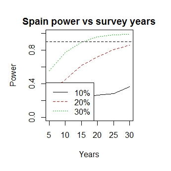
Figure f: A separate power plot for total litter items per BAK haul on the Spanish Coast. The x-axis is the number of years of survey and the different lines represent linear changes in trend
There is moderate confidence in this methodology. There is consensus within the scientific community and the methodology has been used before for this type of assessment and has been published in scientific journals. However it is acknowledged that some aspects require further development, such as inter-comparison between trawl types used in different regions (BAK – GOV) to allow a complete assessment of the relative amounts of litter per km2 to be undertaken.
There is low to moderate confidence in the data availability. The data are a by-product generated by fish stock assessment surveys. There is currently no quality assurance and quality control procedures in place for this data stream, although this will be addressed in the future, and therefore there is some variability in the data quality across some assessment areas (e.g. the English Channel). Also, data have only been collected for the full spatial area covered by the assessment since 2012 so temporal coverage is currently limited, although this will improve with time.
Conclusion
Les déchets sont très répandus sur le sol marin dans l’ensemble des zones évaluées, les déchets plastiques étant prédominants. Dans le cadre des zones évaluées, les quantités de déchets sont plus importantes dans la partie orientale du golfe de Gascogne, les mers Celtiques méridionales et la Manche que dans la mer du Nord au sens large septentrionale et les mers Celtiques septentrionales. Ceci pourrait être dû à des apports anthropiques plus importants, aux fleuves, vents et/ou courants prédominants. Des études antérieures ont révélé que le golfe de Gascogne reçoit de grandes quantités de déchets provenant de fleuves locaux et du transport qui pourrait résulter de la navigation à grande échelle dans l’ensemble de la sous-région. Les déchets flottants et les déchets coulants ont une trajectoire différente et se rassemblent dans des points chauds différents, qui ne chevauchent pas nécessairement. Par exemple, le point chaud pour les déchets sur les plages du Skagerrak ne s’applique pas aux déchets sur le sol marin. Un plus grand nombre de stations ou des séries de données plus longues sont nécessaires pour la plupart des régions OSPAR, à l’exception de la mer du Nord au sens large, afin de pouvoir détecter une modification significative de l’abondance des déchets sur le sol marin. Le Plan d’action régional d’OSPAR détermine des mesures de réduction des déchets marins et devrait permettre une réduction des déchets sur le sol marin.
Lacunes des connaissances
Des connaissances supplémentaires dans certains domaines permettraient d’obtenir une meilleure évaluation. Des informations sur les influences saisonnières, la météorologie et les modifications des courants, pouvant toutes affecter la répartition des déchets, ne sont pas prises en compte. Bien que seules des études utilisant des engins similaires soient utilisées, la conception de l’échantillonnage pourrait également avoir une influence (stations d’échantillonnage fixe ou aléatoire stratifié). De plus, il y a lieu de comparer la méthode de capture des déchets par les divers types d’engin (par exemple chaluts GOV et BAK) si l’on veut comparer à l’avenir des quantités relatives de déchets par km2 dans l’ensemble de la région. Plusieurs problèmes concernant les données ont ralenti l’évaluation et on pourrait améliorer celles-ci au cours des prochaines années.
A longer time series or more survey stations are required to detect trends in individual items or types of litter, therefore these will only be included in future assessments. However, for the Greater North Sea there are sufficient monitoring stations to detect changes of 20% or 30% in seafloor litter abundance, as a result of implemented litter reduction measures. For the Celtic Seas, the Eastern Bay of Biscay, the Iberian Coast and Gulf of Cadiz, there are fewer monitoring stations. An additional 15 to 30 years of monitoring data will be required to predict similar changes (20% or 30% in seafloor litter abundance) in these areas, unless more monitoring stations are added.
To assess the effectiveness of measures through changes in seafloor litter abundance will require more monitoring stations and/or longer data series. Future litter assessments should include modelling to determine sources and pathways. Better knowledge of the fragmentation rates and mechanisms is needed to understand seafloor litter trends and behaviour.
Bergmann, M. & Klages, M. Increase of litter at the Arctic deep-sea observatory HAUSGARTEN. Mar. Pollut. Bull. 64, 2734–2741 (2012).
Bingel, F., Avsar, D., Uensal, M. A note on plastic materials in trawl catches in the north-eastern Mediterranean. Meeresforsch. - Reports Mar. Res. 31, 3–4 (1987).
Carrothers, P. J. G. Estimation of Trawl Door Spread from Wing Spread. J. Northwest Atl. Fish. Sci. 1, 81–89 (1980).
Galil, B. S., Golik, A. & Türkay, M. Litter at the bottom of the sea: A sea bed survey in the Eastern Mediterranean. Mar. Pollut. Bull. 30, 22–24 (1995).
Galgani, F. et al. Distribution and abundance of debris on the continental shelf of the Bay of Biscay and in Seine Bay. Mar. Pollut. Bull. 30, 58–62 (1995a).
Galgani, F., Jaunet, S., Campillo, A., Guenegen, X. & His, E. Distribution and abundance of debris on the continental shelf of the north-western Mediterranean Sea. Mar. Pollut. Bull. 30, 713–717 (1995b).
Galgani, F., Souplet, A. & Cadiou, Y. Accumulation of debris on the deep sea floor off the French Mediterranean coast. Mar. Ecol. Ser. 142, 225–234 (1996).
Galgani, F. et al. Litter on the sea floor along European coasts. Mar. Pollut. Bull. 40, 516–527 (2000).
Galgani, F., Hanke, G., Werner, S. & Vrees, L. De. Marine litter within the European Marine Strategy Framework Directive. ICES J. Mar. Sci. 70, 1055–1064 (2013).
Ioakeimidis, C. et al. A comparative study of marine litter on the seafloor of coastal areas in the Eastern Mediterranean and Black Seas. Mar. Pollut. Bull. 89, 296–304 (2014).
Manly, B. F. J. Randomization, bootstrap and Monte Carlo methods in biology. Texts in statistical science PhD, 455 (2007).
Miyake, H., Shibata, H. & Furushima, Y. Deep-sea litter study using deep-sea observation tools. Interdiscip. Stud. Environ. Chem. 261–269 (2011).
Moriarty, M., Pedreschi, D., Stokes, D., Dransfeld, L. & Reid, D. G. Spatial and temporal analysis of litter in the Celtic Sea from Groundfish Survey data: Lessons for monitoring. Mar. Pollut. Bull. 103, 195–205 (2016).
Pham, C. K. et al. Marine litter distribution and density in European seas, from the shelves to deep basins. PLoS One 9, (2014).
Schlining, K. et al. Debris in the deep: Using a 22-year video annotation database to survey marine litter in Monterey Canyon, central California, USA. Deep. Res. Part I Oceanogr. Res. Pap. 79, 96–105 (2013).
Spengler, A. & Costa, M. F. Methods applied in studies of benthic marine debris. Mar Pollut Bull 56, 226–230 (2008).
Stefatos, A., Charalampakis, M., Papatheodorou, G. & Ferentinos, G. Marine debris on the seafloor of the Mediterranean Sea: Examples from two enclosed gulfs in western Greece. Mar. Pollut. Bull. 38, 389–393 (1999).
Watters, D. L., Yoklavich, M. M., Love, M. S. & Schroeder, D. M. Assessing marine debris in deep seafloor habitats off California. Mar. Pollut. Bull. 60, 131–138 (2010).
Wood SN. Generalized Additive Models: An Introduction with R. Chapman & Hall/CRC; Boca Raton: 2006