

Changes in Phytoplankton Biomass and Zooplankton Abundance
D1 - Biological Diversity D4 - Marine Food Webs
D1.6 - Habitat condition D1.7 - Ecosystem Structure D4.1 - Productivity (production per unit biomass) of key species or trophic groups
Plankton form the base of the marine food web and respond rapidly to environmental changes. Local and large-scale changes in phytoplankton biomass and zooplankton abundance (beyond natural variation) were observed over the period 1958–2002, providing a possible early warning of a wider change in the marine environment.
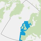
Area assessed
Printable summary
Background
Plankton organisms (both phytoplankton and zooplankton) form the base of the marine food web and are highly sensitive to physical and chemical factors, including nutrient concentration, salinity, and temperature. These factors are dependent on natural variation in climate and hydrography, as well as human-induced processes. Due to their short lifecycles, plankton communities respond rapidly (potentially more rapidly than other trophic levels) to these processes. Plankton-based indicators therefore have the potential to detect those changes at an early stage. Plankton is also essential for organisms higher up the food web, such as shellfish, fish and seabirds, and changes in the plankton community can thus impact on the whole marine ecosystem.
This indicator, based on phytoplankton biomass and zooplankton abundance, provides a means to identify changes (anomalies) in key groups within the plankton community. These changes represent deviations from the assumed natural variability in the plankton time series. The changes are identified as small, important or extreme. This indicator can also help to understand changes in other parts of the marine food web. It has been assessed at two scales: large-scale (ecohydrodynamic regions) and small-scale (coastal stations). When combined with the two other pelagic indicators (that look at changes in plankton lifeform and changes in plankton diversity), it will enable a more sensitive detection of change at the plankton community level.
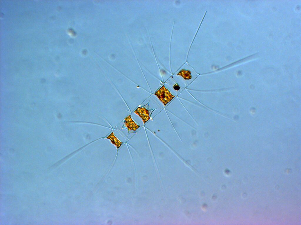
Phytoplankton of the genus Chaetoceros
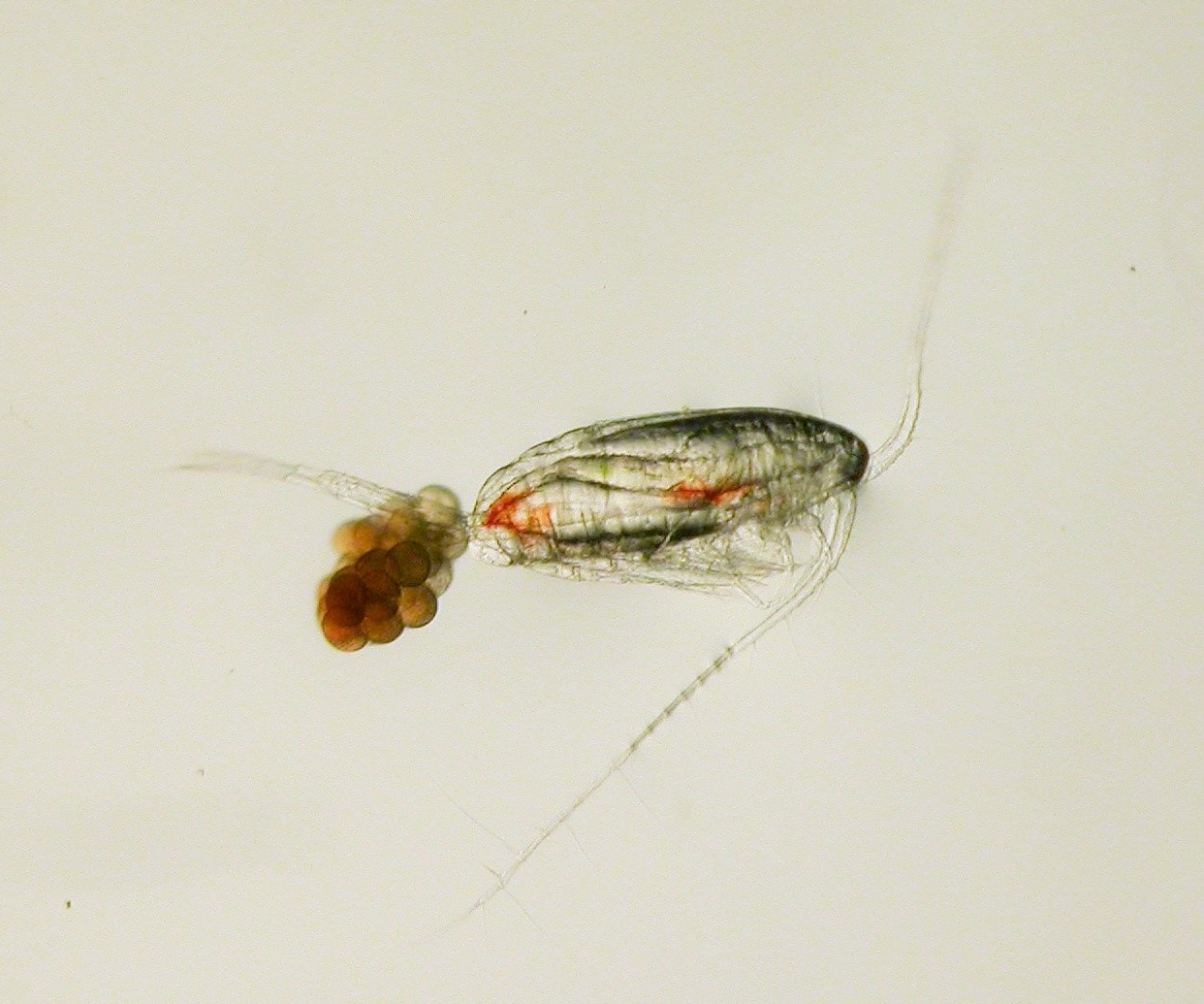
A copepod, the most common type of zooplankton organism (curtesy of Anaïs Aubert)
The amount of marine plankton is, to a large extent, determined by nutrient concentrations, climate and hydrodynamic drivers (e.g. Beaugrand et al., 2009). Total phytoplankton (as biomass using chlorophyll-a or Phytoplankton Colour Index as a proxy) and zooplankton (as abundance - using total copepods abundance) represent key components of the plankton community. They account for the largest part of the plankton biomass and thus having an important role in the whole plankton production, as well as grazing, lysis (auto- and viral), advection and sedimentation processes. Being at the base of the food web, plankton represent (directly or indirectly) a food resource for numerous species at higher trophic levels, such as fish of commercial interest. Variability in phytoplankton biomass and zooplankton abundance can have significant impacts on the structure and function of the marine food web as a whole, as well as on ecosystem processes such as nutrient recycling. The intrinsic characteristics of plankton organisms, such as their small size, lack of commercial exploitation, short lifecycles and a global distribution, render them particularly interesting for monitoring programmes aiming to assess the state of marine ecosystems. Short lifecycles and sensitivity to abiotic factors mean that plankton indicators can provide early warning of change in the marine ecosystem (Batt et al., 2013), from both natural and human-induced change, over a wide range of temporal and spatial scales. Increased pressure on the marine system can be expected to lead to greater and more frequent changes at the base of the food web. Early warning of ecosystem change can help to prompt management actions when changes are still manageable (see Burthe et al., 2016).
A current challenge is to separate expected natural variability from the variability induced by human pressures, a particularly difficult objective that is not yet resolved by plankton science. In the future, further development of this indicator will focus on making the link with human pressures and environmental / climate variability (see Buttay et al., 2015).
Further work is also needed to integrate pelagic habitat indicators (this one, and the indicators on ‘ Changes in Phytoplankton and Zooplankton Communities ’ and ‘ Changes in Plankton Diversity ’) since this will give more confidence in the assessment of plankton changes, and in their integration with indicators of other ecosystem components, in particular food-web indicators.
Robust statistical techniques exist to identify significant components of variation and changes at multiple scales for plankton. These changes may indicate major changes in the marine system involving consequences for other ecosystem components and processes. Significant changes in this indicator are evaluated through time series analysis. One advantage of the methodology is its ease of application to any data set that can be considered ‘long enough’ to represent the temporal variability of plankton. However, since plankton dynamics are not well understood, it is difficult to judge what should be the minimum length of a time series for assessment. As a starting point, it is recommended that minimum time series that should be used is five years, but preferably a minimum ten years. It is also necessary that the monitoring data are acquired at regular intervals through consistent sampling and analytical procedures.
The methodology can be applied to fixed-monitoring station time series (the most frequent situation for monitoring European countries) and to large-scale spatio-temporal data sets such as the Continuous Plankton Recorder (CPR) data or satellite data. The two data types are complementary and may provide information on different temporal / spatial scales and pressures in the future. For instance, coastal data from fixed monitoring stations can be used to identify plankton indicators that could be linked to human pressures, while large-scale spatio-temporal data in the open ocean can be used to define plankton indicators that could be linked to large-scale hydro-meteorological changes or to indirect human pressures (e.g. fishing). An important advantage of these plankton indicators is that the concepts are relatively easily transferable to other regions (Gowen et al., 2011; Rombouts et al., 2013). For the future development of these indicators the definition of reference periods will require knowledge of environmental and human pressure data.
The OSPAR Quality Status Report 2010 highlighted the potential impact of climate change and other human pressures on plankton communities. Phytoplankton chlorophyll-a and phytoplankton indicator species are also assessed under the Common Procedure for the Identification of the Eutrophication Status of the OSPAR Maritime Area (OSPAR Agreement 2013-08) as parameters in problem areas and potential problem areas with regard to eutrophication. There was no comparable regional assessment of phytoplankton biomass and zooplankton abundance.
The full method employed for this indicator is further elaborated in an OSPAR guidance document for both phytoplankton and zooplankton (OSPAR, in prep).
The methodology has been adapted (mainly in the first steps of data preparation) due to the type of data used. First, phytoplankton and zooplankton are considered separately. Second, two main data types related to different acquisition systems are considered here: time series of plankton collected at fixed stations and plankton data from semi-autonomous collecting devices that regularly cover large spatial domains, such as the Continuous Plankton Recorder (CPR) data set.
Pre-analysis Steps: Specificities related to Data Type
Phytoplankton Data
The same approach as for zooplankton applies for total phytoplankton biomass. Instead of looking at a particular species or group, the bulk phytoplankton community is considered through the total phytoplankton biomass. Phytoplankton biomass can be measured as biovolume, carbon content or can be assessed through a proxy, using chlorophyll-a, which is present in all phytoplankton organisms. A semi-quantitative measurement of phytoplankton biomass is also possible by using the so-called Phytoplankton Colour Index (PCI), a method applied on the CPR data. This method estimates the green colour of the plankton community sampled onto a silk net. It should be noted that all data at the large spatial scale used for this indicator assessment originate from the CPR data collection on major shipping routes. Both chlorophyll-a and PCI are used in this assessment as they represent the two types of data regularly monitored in many areas. Chlorophyll-a concentration is already used as an OSPAR common indicator for the assessment of eutrophication.
Zooplankton Data
For zooplankton, only copepods (total copepod abundance) are considered in the calculation. Reduction from total zooplankton abundance to total copepod abundance is justified given that copepods are the best described zooplankton group, consistently determined in samples and are generally the most abundant and ubiquitous zooplankton taxa, both in space and time. In practice, the use of groups, such as copepods, is often favoured over single indicator species. Indeed some species such as meroplankton can have a very patchy distribution and highly variable fluctuation in abundance between years. These fluctuations are often due to natural physical dynamics rather than human pressures (De Jonge, 2007). An indicator based on only one species is also unlikely to represent the whole trophic level to which it belongs and which is required here for the present indicator assessment. To use a group as large as copepods allows the comparison of most of the zooplankton time series which can bring valuable understanding to the plankton dynamic.
Thus, as a first step, all copepod species abundance per time unit (sample) must be summed.
Non-station Data
For the CPR time-series, and large spatio-temporal pelagic data sets in general, the first step is geographic sub-division. Pelagic habitat boundaries are not fixed and are characterized by high spatio-temporal dynamics. Deciding on the geographic sub-divisions involved preparatory work on the identification of eco-hydrodynamic zones, which in turn required physico-chemical data. For the Greater North Sea region and the Celtic Seas region, this type of work has been undertaken by Van Leeuwen et al. (2015) who defined five ecohydrodynamic zones (EHDs) (and one undefined zone) (Figure a). The model is however weaker for the Celtic Seas region. For the Bay of Biscay and Iberian Coast region, preliminary work has been undertaken in France identifying 10 EHDs (Gaillard-Rocher et al., 2012). The raster image for dividing the Bay of Biscay and Iberian Coast region into EHDs was not available at the time of this assessment.
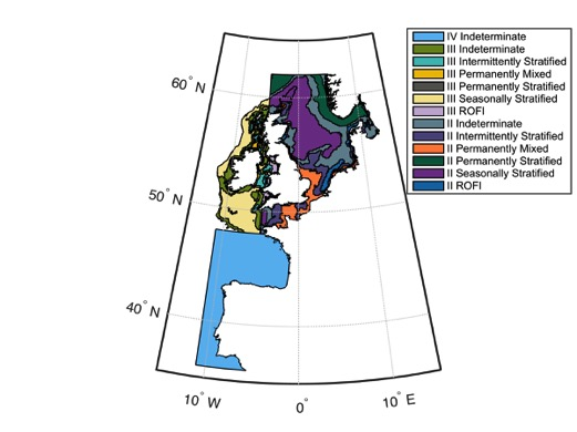
Figure a: Ecohydrodynamic zones (EHDs) in the Greater North Sea, Celtic Seas, and the Bay of Biscay and Iberian Coast
EHDs are constructed based on key water column features, which are important to plankton community structure and dynamics. Based on water column structure, there are six predominant EHD types: permanently mixed throughout the year; permanently stratified throughout the year; regions of freshwater influence (ROFIs); seasonally stratified (for about half the year, including summer); intermittently stratified; and indeterminate regions (inconsistently alternate between the above levels of stratification). Work is on-going to define ecohydrodynamic zones in the Bay of Biscay and Iberian Coast.
Raster images necessary for dividing the CPR data from the Greater North Sea and Celtic Seas into EHDs have been produced based on the work of Van Leeuwen et al. (2015) and make it possible to sub-divide the larger area (Greater North Sea and Celtic Seas) into EHDs with the R script provided in this assessment (R is a programming language that allows fast calculation) (Stephen, D. and Lynam, C. (Cefas) pers. comm.). The script can be applied to any data set in the Greater North Sea and Celtic Seas as long as the longitude and latitude coordinates of the samples are known. The R script has been provided as supplementary information associated with this assessment.
Recommendations for precision are written within the script. One of the main considerations is that years missing more than four months of data should be omitted when running the analysis (to avoid bias in the analysis).
For the Greater North Sea, the correspondence between EHDs and the raster file supplied is as follows: 1 (permanently stratified), 2 (seasonally stratified), 3 (permanently mixed), 4 (regions of freshwater influence; ROFI), 5 (intermittently stratified) and 6 (not defined).
For the Celtic Seas, the correspondence between EHDs and the raster file supplied is as follows: 1 (seasonally stratified), 2 (permanently stratified), 3 (regions of freshwater influence; ROFI), 4 (permanently mixed) and 5 (intermittently stratified).
The coordinates for the CPR samples cannot be provided due to data sharing restrictions. The CPR data set is owned by the Sir Alister Hardy Foundation for Ocean Science (SAHFOS).
Calculation of monthly means
After the data have been fitted to the correct geographic scale, and before running the time series analysis, the data were averaged per month over the whole time series. This needs to be done for each data set independently of the type of data.
Data provided and used in this assessment
The CPR total copepod data for the Greater North Sea and Celtic Seas have been provided per EHD (based on Van Leeuwen et al., 2015). For the Celtic Seas, some EHDs did not contain enough data to run the analysis and so have been excluded. For phytoplankton, the assessment has been made per EHD for the Greater North Sea but not for the Celtic Seas due to time constraints. The assessment for the Bay of Biscay and Iberian Coast is done at the OSPAR-region level, for both phytoplankton and zooplankton.
Fixed-station data were provided by Denmark, France, Germany, Spain, Sweden and the United Kingdom. However, due to limited time and resources available, only some station data have been used in this assessment (those from France, Sweden and one for the United Kingdom). Other data are available (those for Danish and German stations and will be assessed in the next cycle).
The data used for this assessment are as follows.
Phytoplankton:
- CPR PCI data for the Bay of Biscay and Iberian Coast region for the period 1958–2013;
- CPR PCI data for the Greater North Sea for all EHDs for the period 1958–2012;
- CPR PCI data for the Celtic Seas for the period 1958–2012;
- Chlorophyll-a data for the L4 station (United Kingdom) for the period 2001–2013;
- Chlorophyll-a data for the French SOMLIT Wimereux coastal (C) and offshore (L) stations for the period 1998–2013;
- Chlorophyll-a data from the Swedish station Släggö Skagerrak for the period 1990–2014; and
- Chlorophyll-a data from the Swedish station Anholt E, Kattegat for the period 1983–2015.
Zooplankton:
- CPR total copepod abundance for the Greater North Sea for all EHDs for the period 1958–2012;
- CPR total copepod abundance for the Celtic Seas, for the seasonally and intermittently stratified waters for the period 1958–2012 and for the ROFIs for the period 1971–2012;
- CPR total copepod abundance for the Bay of Biscay and Iberian Coast region for the area as a whole for the period 1958–2012; and
- Total copepod abundance for two Swedish stations: Anholt E for the period 2003–2013 and a more coastal station, N14 Falkenberg for the period 2008–2013.
Methodology and concepts
The present indicator assessment is based on robust and basic time series analysis, identifying anomalies. Anomalies represent deviations from the assumed natural variability of the time series (following further development, future assessments could examine deviation from a reference period). The longer a time series, the more suited it is for assessing natural variability. It is difficult to assess natural variability using short time series. The greater the anomaly (in terms of absolute value, since anomalies can be positive or negative), the greater the change in metric (here, phytoplankton biomass or zooplankton abundance). An anomaly value of zero means there is no anomaly, and thus zero represents the time series mean (which must be de-seasonalised).
Two types of anomaly are produced in this analysis: annual anomalies and monthly anomalies. The former are presented in this assessment. However, to understand the changes presented (i.e. annual anomalies) and to be most useful for decision makers, the annual anomalies must be considered using details given by the monthly anomalies (since an early warning indicator should be assessed at the best temporal resolution possible).
Anomalies are calculated for both the phytoplankton and zooplankton data. The time series analysis used was developed in R for the plankton time series by Ibanez (reported in Berline et al., 2009), and then adapted for use in this assessment.
Please note that the R script has been applied to PCI data, however due to the mathematical properties of the PCI, semi-quantitative counts transformation, it might be that the time-analysis has to be revised and adapted for use with the PCI data.
The anomalies are categorised in order to improve the presentation of these results from a graphical perspective and to simplify the results for use in management. The categorisation is based on percentiles; the 2.5-, 25-, 50-, 75- and 97.5-percentiles have been used to categorise the anomalies within a time series. Three categories are used: small change (anomalies within the 25–75 percentile range), important change (anomalies within the 2.5–25 percentile range and 75–97.5 percentile range) and extreme change (anomalies within the 0–2.5 percentile range and 97.5–100 percentile range).
Three colours have been attributed to each category: light blue (small change), blue (important change) and dark blue (extreme change).
Anomalies within the small change category represent the scenario least likely to represent significant shifts at the plankton community level and thus to impact on the marine ecosystem. Anomalies within the important change and extreme change categories have increasing potential to represent significant modification of the plankton community and thus to impact on the marine ecosystem. This initial categorization will be further discussed in the future, with potential changes and improvements.
Because annual anomalies are averaged by year, they may reflect a mix of positive and negative anomalies, which are qualified overall as small change rather than presenting a strong anomaly signal identified for a certain period. This should be carefully considered when interpreting the results. More detailed interpretation can be informed by examining the monthly anomalies.
In the future, the methodology could be strengthened by identifying clear regime shifts, in addition to anomalies. Analytical tools exist for plankton regime shift analysis and will be considered in the future development of this indicator.
As highlighted in the three assessment sheets for pelagic indicators, each pelagic habitat indicator considers the plankton community at a different level of organisation: the lifeform indicator at the functional level of the community; the present indicator on total biomass / abundance at the level of aggregated community properties; and the plankton diversity indicator at the species and community structure levels. By combining the information from these three state indicators, a more holistic assessment of plankton dynamics can be obtained than from each indicator individually. The pelagic indicators are intended to be used as a suite, to give more confidence and power to the pelagic habitat assessment and to strengthen the power to detect change. The goal is to have indicators which can be used as ‘early warnings’ of ecosystem and biodiversity changes.
Time Series Analysis
The time series analysis, run with an R script is the same for any type of data, both fixed-station data and CPR data, and phytoplankton and zooplankton data, as long as the pre-analysis steps have been followed (the step of creating monthly averages is provided as a separate R script). When the data are in the form of monthly means (the data have to be under the same format originally), the time series analysis can be run. The script is provided with comments and in a step-order as it is commonly done for an R script.
Results
This assessment identifies changes in plankton communities at both the large scale and local scale. At the large geographic scale, this is illustrated by the assessment of the ecohydrodynamic (EHD) zone ‘intermittently stratified waters’ of the Greater North Sea. Figure 1 shows the results for phytoplankton biomass and Figure 2 for zooplankton abundance. The graphics show annual deviations from the assumed natural variability (anomalies) of the time series for the period 1958–2012. Such anomalies can be positive or negative with the magnitude of the change being split into three categories (small change, important change or extreme change).
For phytoplankton, the time-series can be subdivided into four main periods (Figure 1). From the start of the time-series (1958) to around 1965, most anomalies are negative and qualified as important changes. The period 1965-1975 then appears relatively stable and characterised by small changes in phytoplankton biomass. From 1975, a decrease occurred with mostly negative anomalies, categorised as important changes in phytoplankton biomass. In fact, this period is recognised as marking a regime shift in the North Sea. The phytoplankton biomass after 1985 and up to 2012 mostly exhibits positive anomalies categorised as small and important scale change, with very few exceptions. The anomalies increase in strength, and are qualified as important, between 2010 and 2012.
For zooplankton, the time-series of annual anomalies shows five main periods between 1958 and 2012 (Figure 2). The time-series exhibits positive anomalies representing extreme change at the start (1958-1959) followed by a period with positive anomalies showing important and small change, between 1960-1972. After 1970, we see mostly negative anomalies and categorise these as important changes with some notable extreme negative anomalies around 1980. This shows a clear decrease in zooplankton abundance over this period. This period also corresponds to a well-known regime shift and fish stock decline in the North Sea. From 1982 to 2006, zooplankton abundance increased with mostly positive anomalies exhibited, and with some important changes, up to the mid-1990s. Subsequent anomalies are negative, and start to be for most of them, qualified as important changes from 2004 to 2012 showing a decrease in zooplankton abundance. The results tend to show that for this EHD zone (intermittently stratified waters) and for the known regime shift of the early 1980s, that zooplankton abundance exhibits stronger negative anomalies than phytoplankton biomass. For the most recent period after 2000, the results show two opposing tendencies: zooplankton abundance tending to decrease while phytoplankton biomass tended to increase. These results need to be related to knowledge about environmental variability and human pressures in order to fully interpret them.
There is moderate confidence in the methods and data used in this assessment.
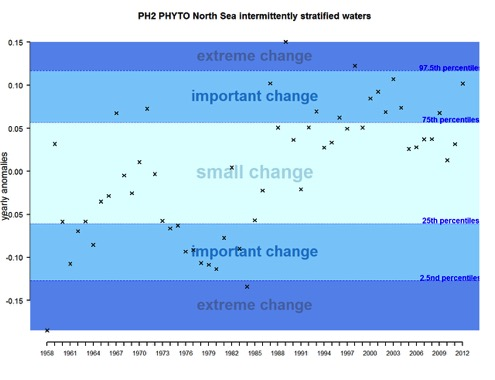
Figure 1: Annual anomalies for phytoplankton biomass for the Greater North Sea for intermittently stratified waters over the period 1958–2012
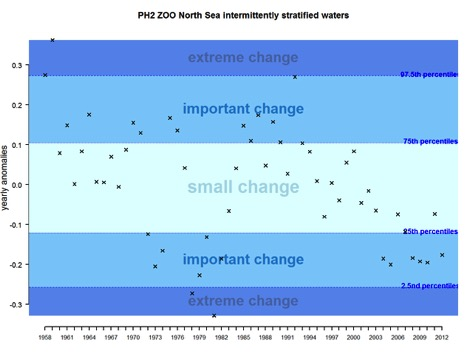
Figure 2: Annual anomalies for zooplankton abundance for the Greater North Sea for intermittently stratified waters over the period 1958–2012
The results of annual anomalies are available for several ecohydrodynamic zones (EHDs) in the Greater North Sea (Figures b-f and m-q) and the Celtic Seas (Figures g, r, s), as well as for the Bay of Biscay and Iberian Coast (Figures h, t) as a whole. Results for phytoplankton biomass are also available for one station in the United Kingdom (L4, Figure k), one in Sweden (Slaggo, Figure l) and two in France (inshore and offshore Wimereux, Figures i, j). Results for zooplankton abundance are also available for one United Kingdom station, and two Swedish stations (Anholt and N14 Falkenberg (Figure u, v)). All these results show that most datasets exhibit strong variability over time in term of anomalies. All data sets exhibit some years of extreme change and important change. However, it is important to stress that the categorisation of the anomalies is strongly dependent on the length of the time series. The shorter a time series, the less confidence there is in the categorisation of its anomalies since the natural variability is known only over a limited period of time. Thus, for fixed stations, the data must be interpreted with more caution due to the shorter length of the time series. The results of this assessment are able to show the main patterns in change, and can be used as ‘early warnings’. For instance, if a recent year is categorised as showing extreme change (either in a positive or negative direction), it highlights that particular year should be further investigated. Where years are showing strong anomalies in the important and extreme categories, the monthly anomalies would be useful to identify if this result is linked to seasonal variability. This is useful for the other biological compartments and food-web indicators, since important changes found in other descriptors can be compared with those found for the biodiversity indicators.
Confidence Assessment
The methodology and approach of the Changes in Phytoplankton Biomass and Zooplankton Abundance indicator is widely accepted and is used in published peer-reviewed literature, but progress still needs to be made in determining reference periods to aid interpretation. The assessment is undertaken using data with a mostly sufficient spatial and temporal coverage for the area assessed, but gaps are apparent in certain areas, especially coastal areas. In-situ data from additional Contracting Parties need to be included. Therefore the data and methods used are considered robust and of moderate confidence.
For Phytoplankton:
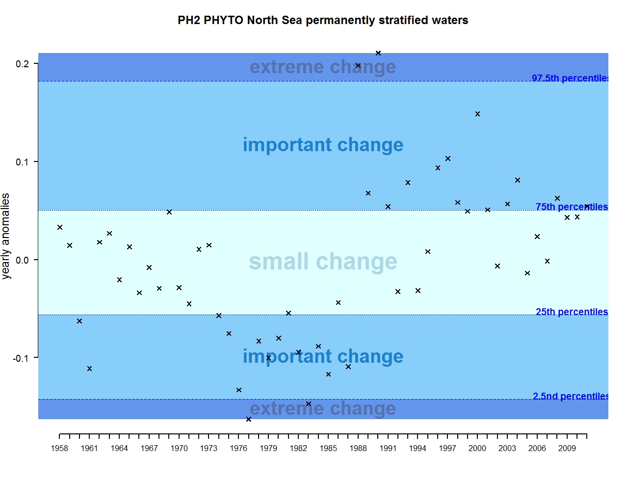
Figure b: Annual anomalies in phytoplankton biomass for the permanently stratified waters of the Greater North Sea
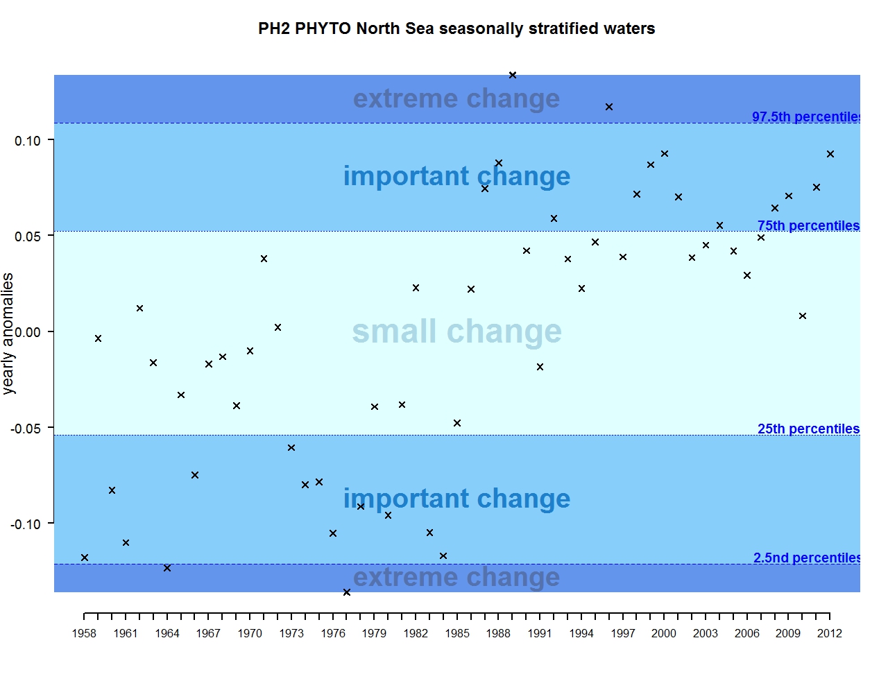
Figure c: Annual anomalies in phytoplankton biomass for the seasonally stratified waters of the Greater North Sea
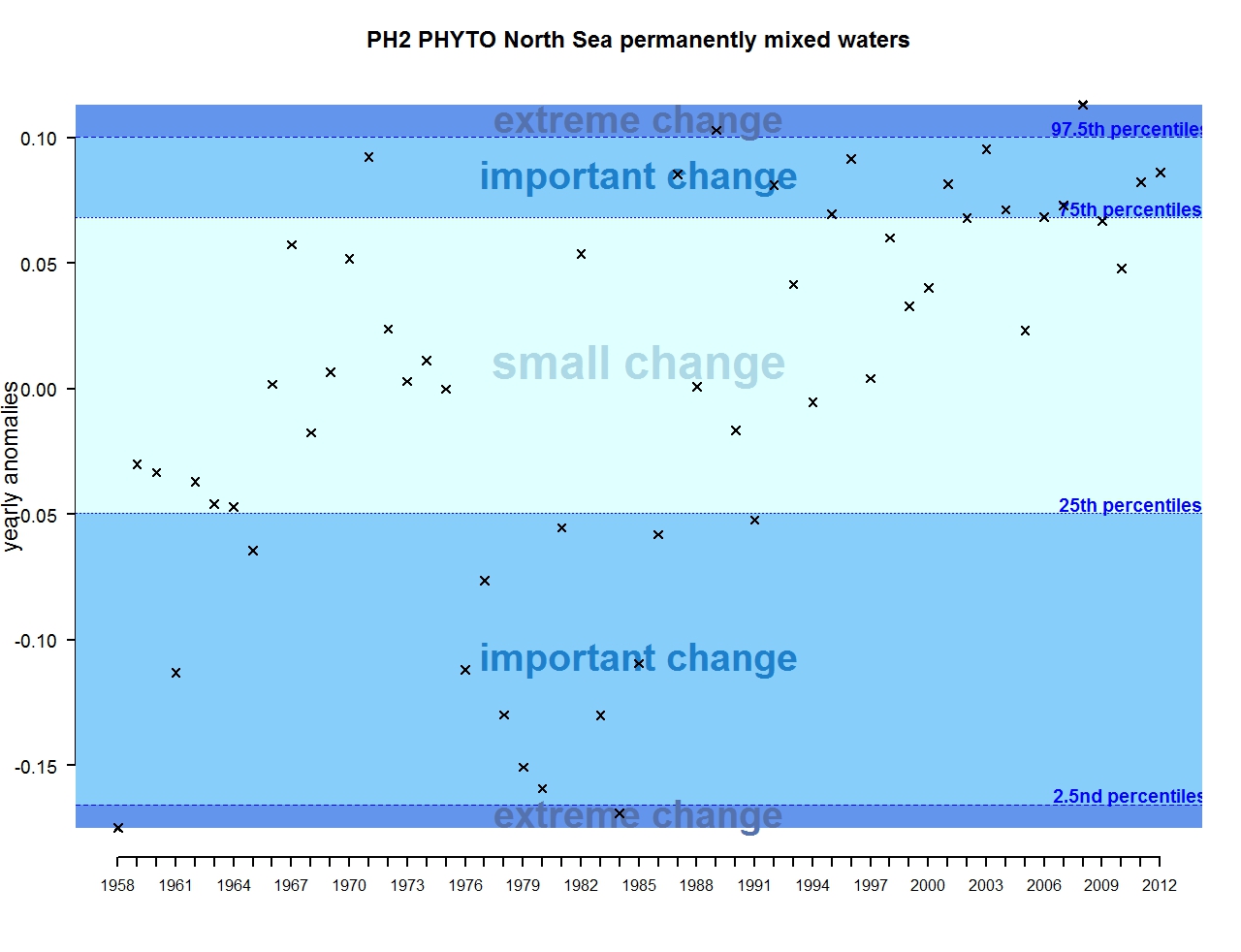
Figure d: Annual anomalies in phytoplankton biomass for the permanently mixed waters of the Greater North Sea
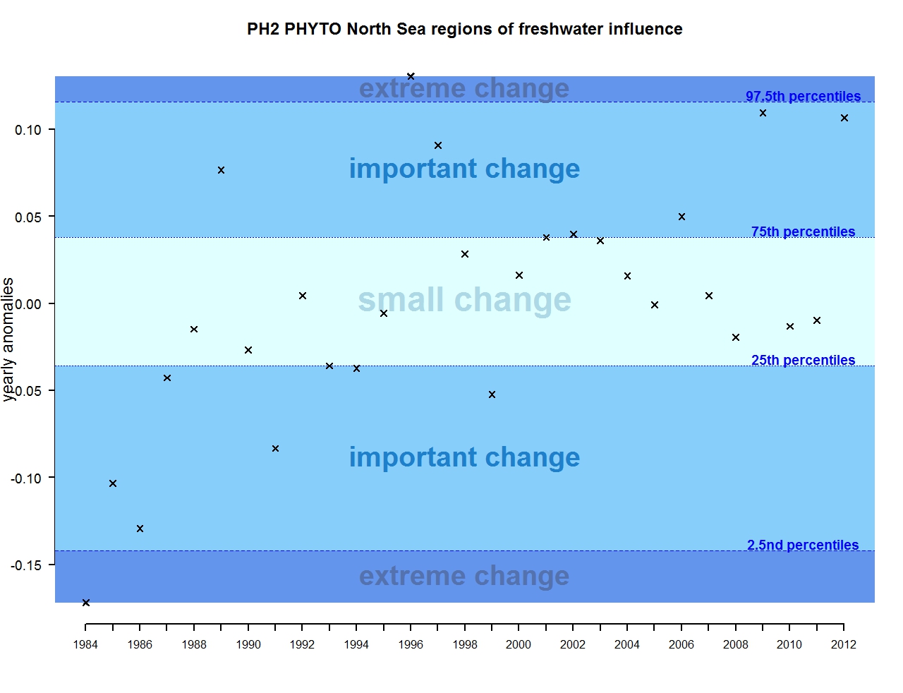
Figure e: Annual anomalies in phytoplankton biomass for the regions of freshwater influence in the Greater North Sea
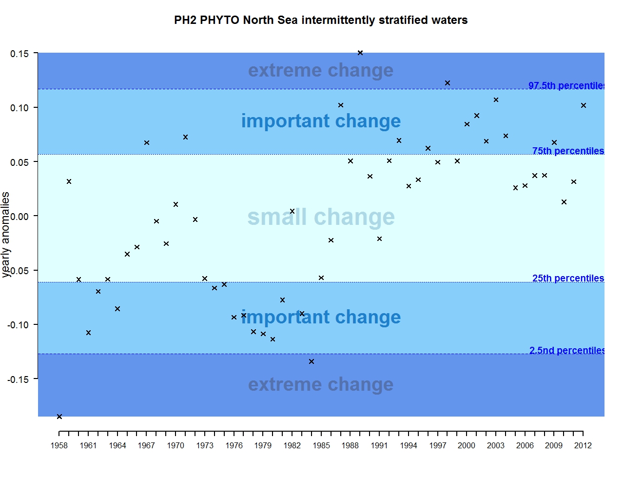
Figure f: Annual anomalies in phytoplankton biomass for the intermittently stratified waters of the Greater North Sea
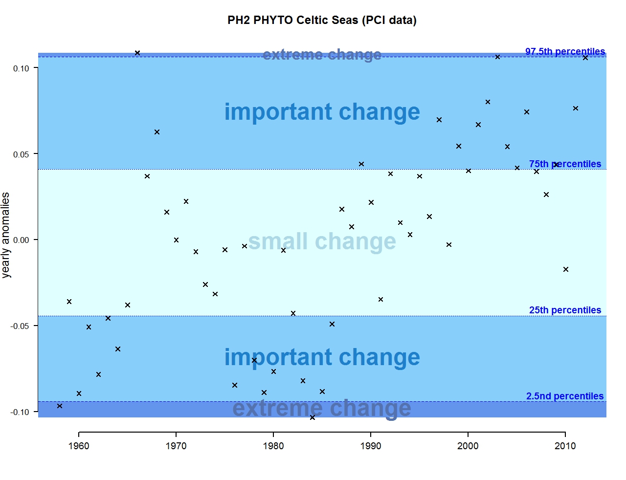
Figure g: Annual anomalies in phytoplankton biomass for the Celtic Seas
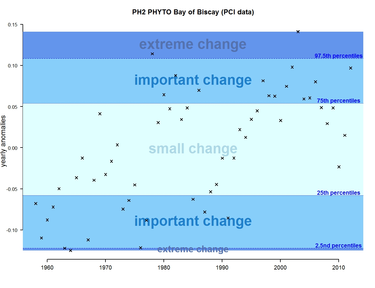
Figure h: Annual anomalies in phytoplankton biomass for the Bay of Biscay and Iberian coast
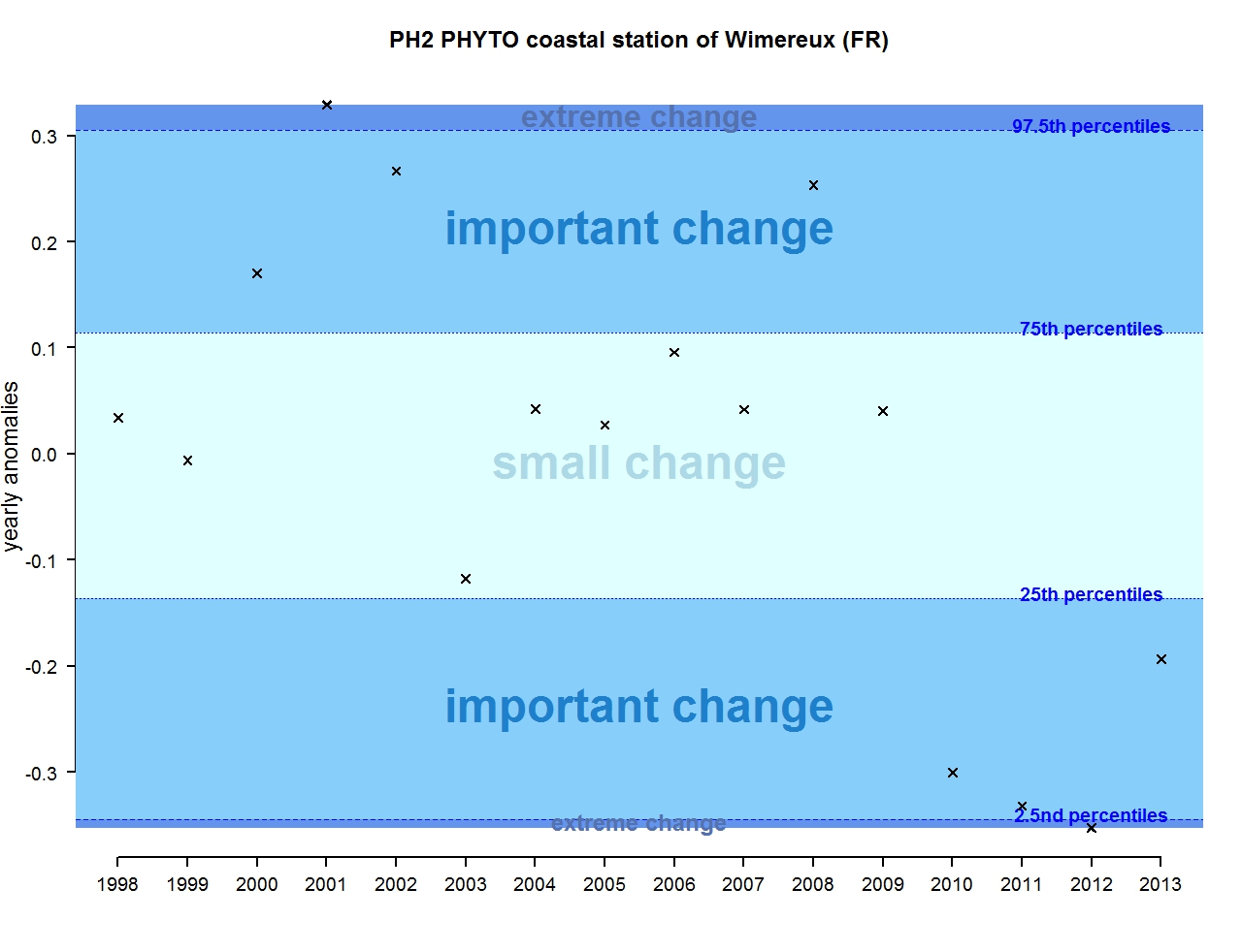
Figure i: Annual anomalies in phytoplankton biomass for the coastal station of Wimereux
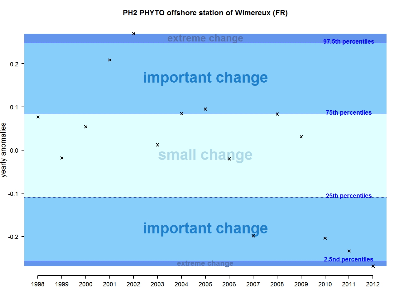
Figure j: Annual anomalies in phytoplankton biomass for the offshore station of Wimereux
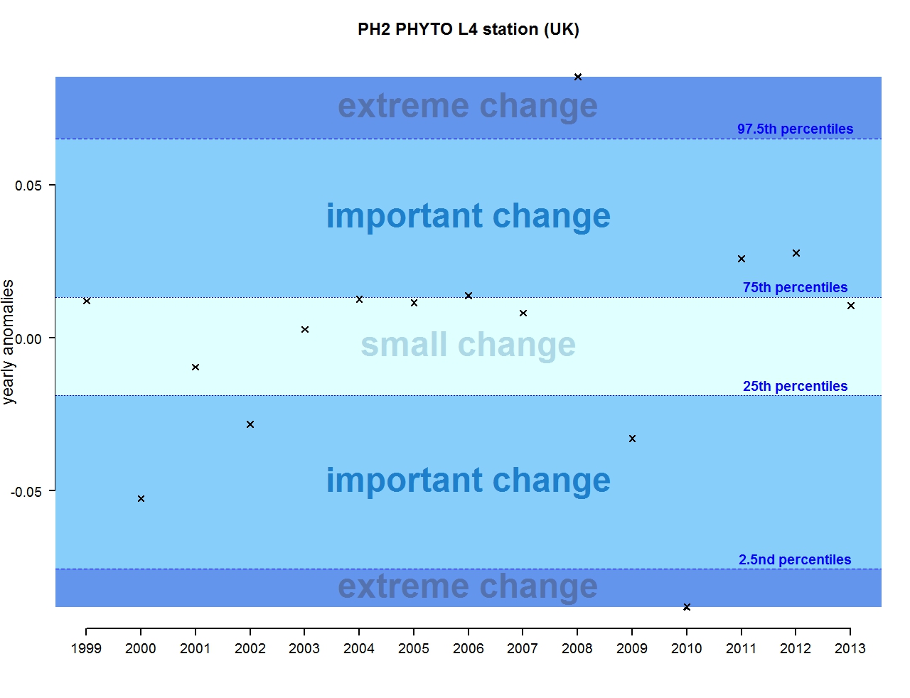
Figure k: Annual anomalies in phytoplankton biomass for the L4 station
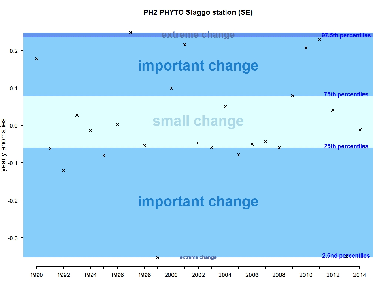
Figure l: Annual anomalies in phytoplankton biomass for the Swedish station Slaggo
For Zooplankton
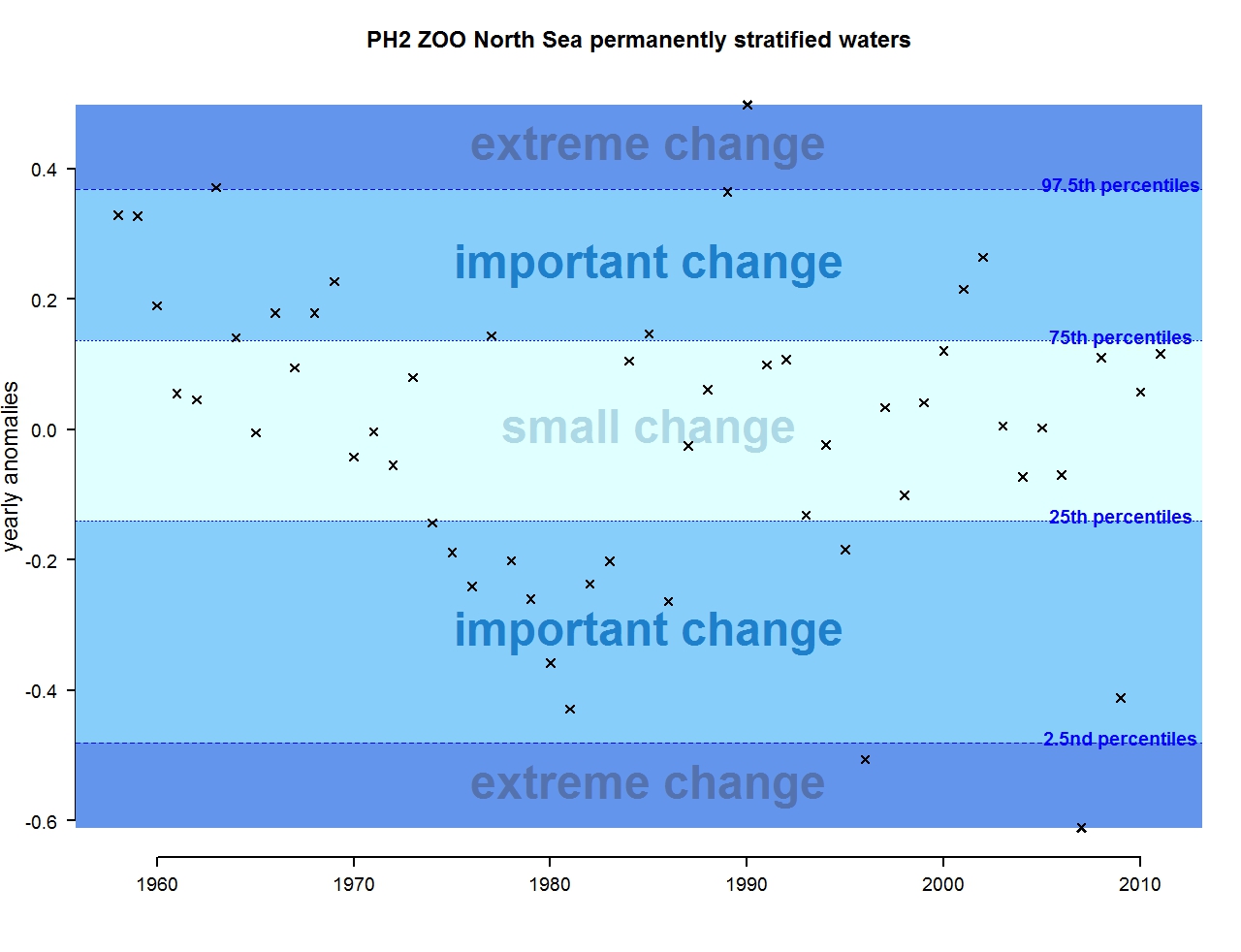
Figure m: Annual anomalies in zooplankton abundance for the Greater North Sea for the permanently stratified waters
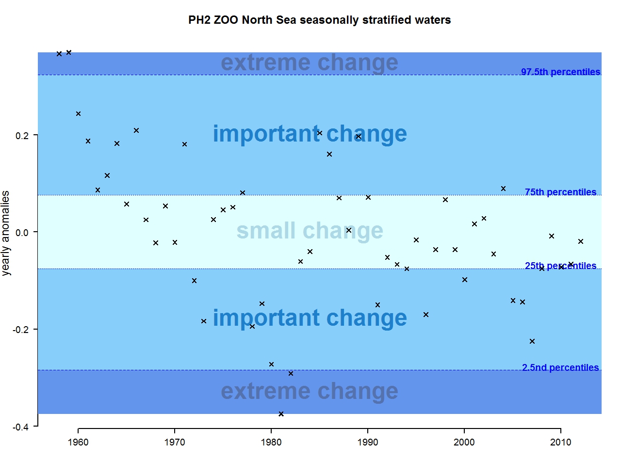
Figure n: Annual anomalies in zooplankton abundance for the Greater North Sea for the seasonally stratified waters
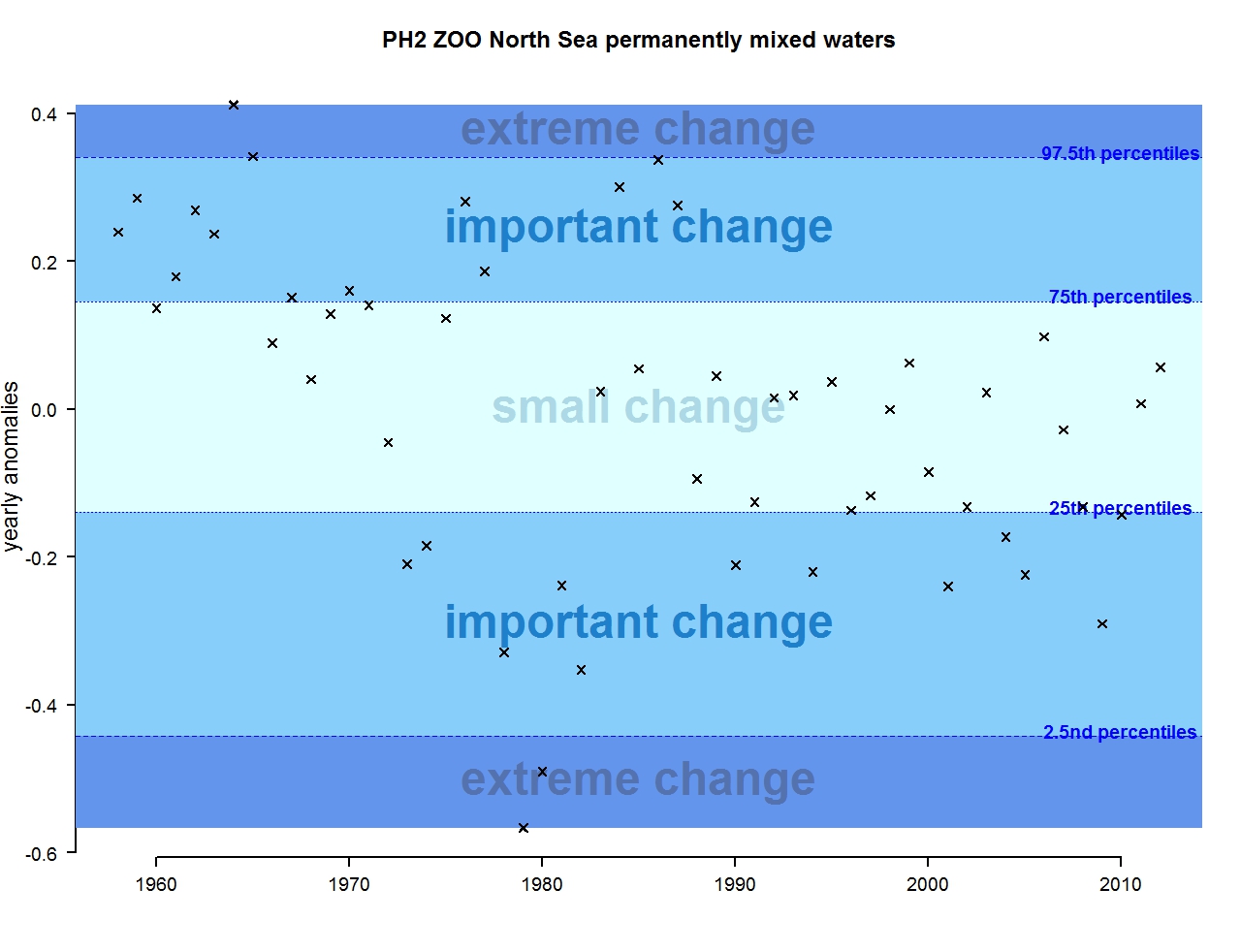
Figure o: Annual anomalies in zooplankton abundance for the Greater North Sea for the permanently mixed waters
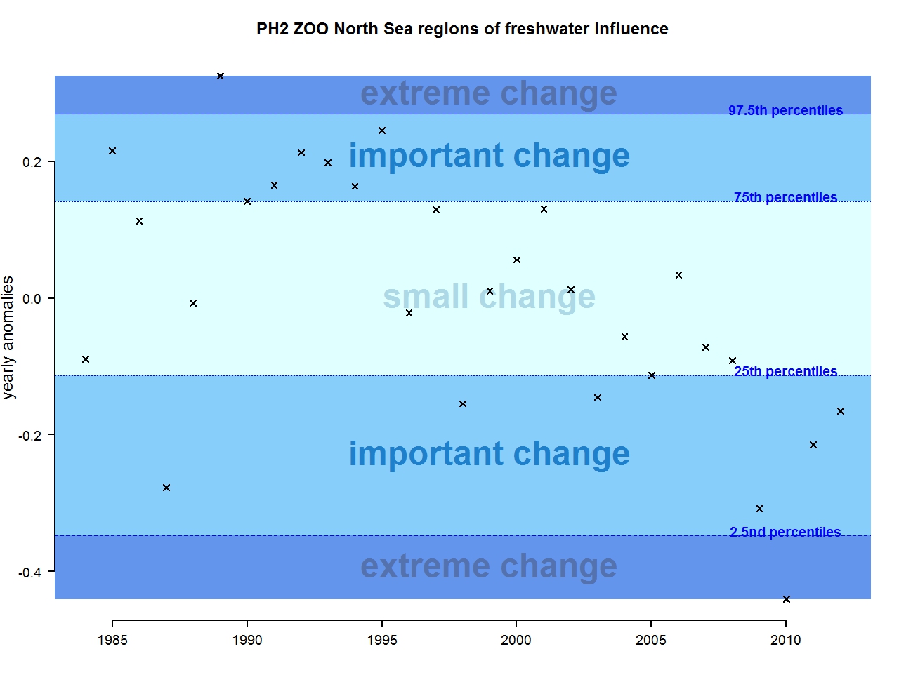
Figure p: Annual anomalies in zooplankton abundance for the Greater North Sea for the regions of freshwater influence
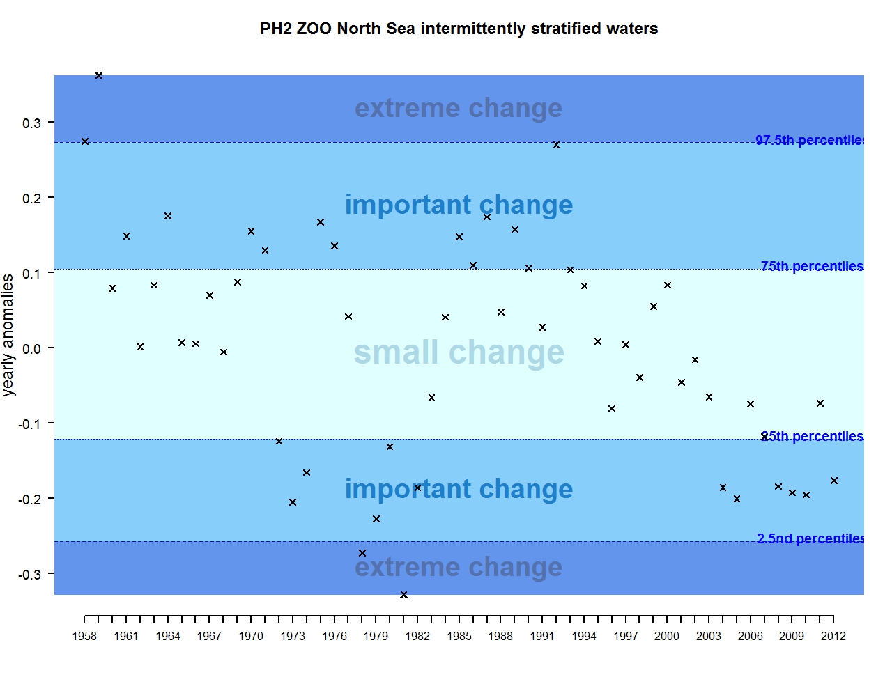
Figure q: Annual anomalies in zooplankton abundance for the Greater North Sea for the intermittently stratified waters
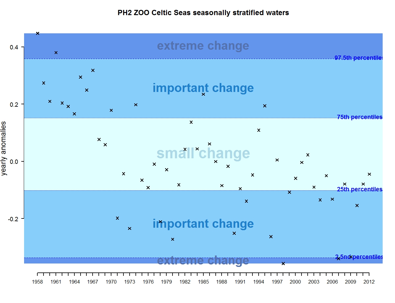
Figure r: Annual anomalies in zooplankton abundance for the Celtic Seas for the seasonally stratified waters
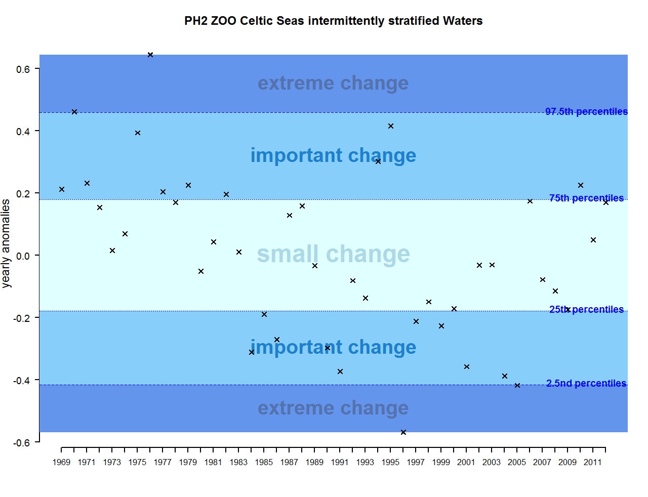
Figure s: Annual anomalies in zooplankton abundance for the Celtic Seas for the intermittently stratified waters
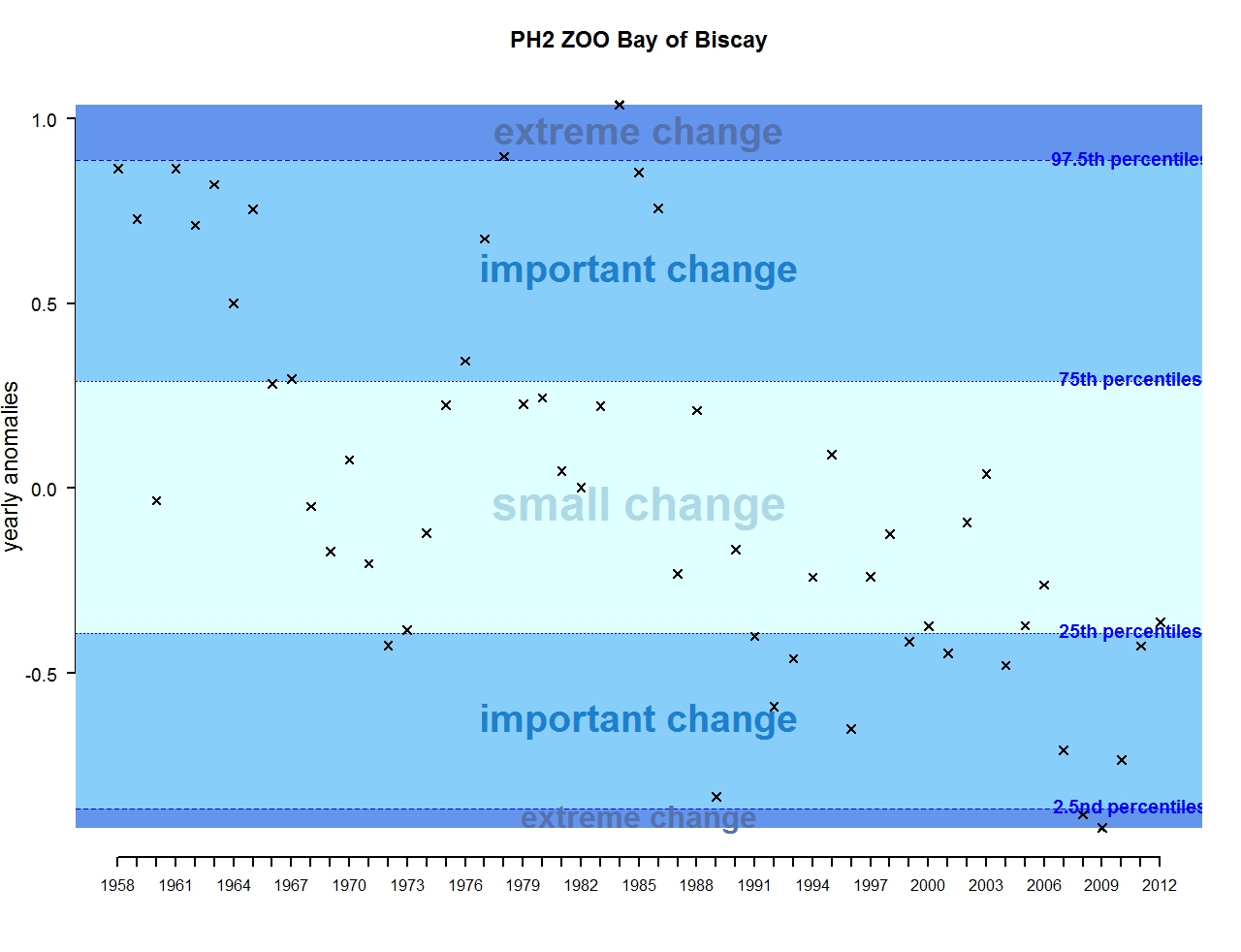
Figure t: Annual anomalies in zooplankton abundance for the Bay of Biscay and Iberian coast
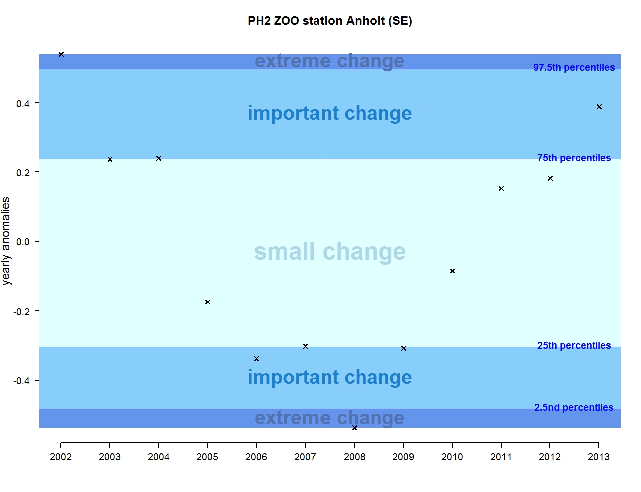
Figure u: Annual anomalies in zooplankton abundance for the Swedish station Anholt
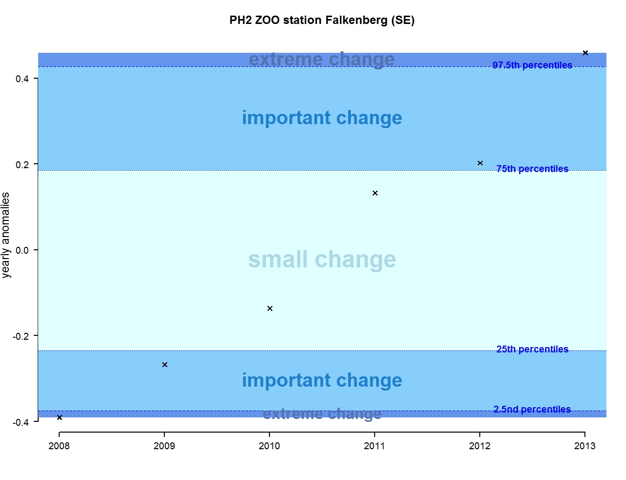
Figure v: Annual anomalies in zooplankton abundance for the for the Swedish station N14 Falkenberg
Conclusion
This indicator shows the variation in phytoplankton biomass and zooplankton abundance for large geographic areas (ecohydrodynamic zones and entire OSPAR regions) and some small scale coastal stations. The indicator is based on the identification of changes calculated through time-series anomalies of phytoplankton biomass (chlorophyll-a and Plankton Colour Index) and zooplankton abundance (total copepod abundance).
The assessment is preliminary and shows that important scale changes occurred, acting as an early warning and flagging a potential issue for the wider marine ecosystem.
Knowledge Gaps
Further work recommendations are as follows: 1. Further interpretation of the results in detail, considering monthly anomalies and scientific knowledge expertise of the studied geographical assessment unit; 2. Link with environmental and anthropogenic pressure data to interpret the changes; and 3. Definition of reference periods related to GES (Good Environmental Status).
Several of the following gaps in the assessment have been partly addressed during the European Union co-financed EcApRHA project:
The integration of the plankton indicators to provide a more holistic perspective of the dynamics of the plankton community, based on a case study (L4 station, United Kingdom).
Further development of this indicator is needed, particularly on these points:
- Inclusion of additional existing data sets, both at the large geographic scale and for coastal stations; the need to sub-divide the Bay of Biscay and Iberian Coast region into ecohydrodynamic zones;
- Assessment of the link with environmental variables (such as temperature and salinity) and human pressures; and
- Definition of reference periods for each assessment unit in relation to environmental and human pressures data, and to scientific knowledge of the area.
Inclusion of Additional Datasets
There are many existing datasets that have not been used in this assessment owing to non-accessibility. Accessibility of data, as well as adequate quality and format, should be ensured. This should be a focus for the next cycle of assessment of OSPAR indicators. The development of a common database would help this process. For phytoplankton, only chlorophyll-a and Phytoplankton Colour Index (PCI) are used for this indicator assessment but other proxies of chlorophyll-a such as satellite chlorophyll estimations or in vivo fluorescence data could also be used and could help in considering a wider spatial and temporal coverage.
Future research and monitoring studies should address the various gaps in monitoring data coverage, particularly at the large scale, because these will be a limiting factor for the development of the indicators in the future. Semi-automated methods such as in vivo multi-spectral fluorometry and flow cytometry (Houliez et al., 2012; Bonato et al., 2015; Thyssen et al., 2015), supplemented by automated image acquisition and analysis which allow higher spatial and temporal resolution should also be considered within the monitoring programmes. This has been developed as part of the EcApRHA deliverables (Aubert et al., 2017) and recommendations have been made for the further development of the pelagic habitat indicators. Such methods can also provide information on additional aspects of the plankton community (such as size class and analysis of smaller organisms) that can be useful for the calculation of the other plankton indicators.
Sub-dividing the Bay of Biscay and Iberian Coast into Ecohydrodynamic Zones
Recommendations on sub-dividing the Bay of Biscay and Iberian Coast into ecohydrodynamic zones are made in the Action Plan of the EcApRHA project.
Assessing the Link with Environmental Variables and Human Pressures
In order to fully understand the changes identified in this assessment, the results must be combined with environmental and pressure data. Past and present environmental and human pressure data need to be acquired. Further development will involve incorporating more data sets and interpreting the new results obtained, in order to inform management decisions. Recommendations on this issue are made in the Action Plan of the EcApRHA project.
Defining Reference Periods Related to Good Environmental Status
The present time-series analysis treats the totality of the time series, and no reference periods have been set up. As such, the plankton indicator can only be considered a ‘state indicator’ because it is unable to relate the changes identified to a future Good Environmental Status (GES). Once reference periods are defined it should be possible to determine GES. Establishing reference periods will require that environmental and human pressure data are made available, as well as specific area knowledge provided by experts. Recommendations on this issue are made in the Action Plan of the EcApRHA project.
Aubert A., Rombouts I., Artigas F., Budria A., Ostle C., Padegimas B., McQuatters-Gollop A. 2017, “Combining methods and data for a more holistic assessment of the plankton community”, as a contribution to the EU Co-financed EcApRHA project (Applying an ecosystem approach to (sub) regional habitat assessments), deliverable No. 1.2.
Batt, R.D., Brock, W.A., Carpenter, S.R., Cole J.J., Pace M.L., Seekell D.A., 2013. Asymmetric response of early warning indicators of phytoplankton transition to and from cycles. Theor Ecol., 6: 285. doi:10.1007/s12080-013-0190-8
Beaugrand G, Luczak C, Edwards M (2009) Rapid biogeographical plankton shifts in the North Atlantic Ocean. Glob Change Biol 15:17901790ift
Berline L., Ibanez F., Grosjean P. 2009. Roadmap for zooplankton time series analysis. SESAME WP1 report. 20p.
Bonato, S., Christaki, U., Lefebvre, A., Lizon, F., Thyssen, M., Artigas, L.F. (2015). High spatial variability of phytoplankton assessed by flow cytometry, in a dynamic productive coastal area, in spring:the eastern English Channel. Estuarine Coastal And Shelf Science, 154, 214-223.
Burthe, S. J., Henrys, P. A., Mackay, E. B., Spears, B. M., Campbell, R., Carvalho, L., Dudley, B., Gunn, I. D. M., Johns, D. G., Maberly, S. C., May, L., Newell, M. A., Wanless, S., Winfield, I. J., Thackeray, S. J. and Daunt, F. 2016. Do early warning indicators consistently predict nonlinear change in long-term ecological data?. J Appl Ecol, 53: 666–676. doi:10.1111/1365-2664.12519
Buttay L., Miranda A., Casas G., González-Quirós R., Nogueira E. 2015. Long-term and seasonal zooplankton dynamics in the northwest Iberian shelf and its relationship with meteo-climatic and hydrographic variability. J. Plank. Res. doi:10.1093/plankt/fbv100
De Jonge V.N. 2007. Toward the application of ecological concepts in EU coastal water management. Marine Pollution Bulletin 55, 407-414.
Gaillard-Rocher I.,Huret M., Lazure P., Vandermeirsch F., Gatti J., Garreau P., Gohin F. 2012. Identification de “paysages hydrologiques” dans les eaux marines sous juridiction française (France métropolitaine). Ifremer report, 48p.
Gowen R.J., McQuatters-Gollop A., Tett P.M., Bresnan E., Castellani C., Cook K., Forster R., Scherer C., Mckinney A. 2011. The Development of UK Pelagic (Plankton) Indicators and Targets for the MSFD, Belfast, 2011.
Houliez, E., Lizon F.,Thysse N.M., Artigas L.F. and Schmitt F.G. 2012. Spectral fluorometric characterization of Haptophyte dynamics using the FluoroProbe: an application in the eastern English Channel for monitoring Phaeocystis globosa. J. Plankton Res.34:136-151
OSPAR (in prep). OSPAR Agreement 20xx-x. Coordinated Environmental Monitoring and Assessment Programme Guidelines for assessing changes in phytoplankton biomass and zooplankton abundance. www.ospar.org
Rombouts I., Beaugrand G., Fizzala X., Gaill F., Greenstreet S.P.R., Lamare S., Le Loc’h F., McQuatters-Gollop A., Mialet B., Niquil N., Percelay J., Renaud F., Rossberg A.G. and Féral J.P., 2013. Food web indicators under the Marine Strategy Framework Directive: from complexity to simplicity? Ecological Indicators, 29: 246–254.
Thyssen, M., Alvain, S., Lefèbvre, A., Dessailly, D., Rijkeboer, M., Guiselin, N., Creach, V., and Artigas, L.-F. (2015) High-resolution analysis of a North Sea phytoplankton community structure based on in situ flow cytometry observations and potential implication for remote sensing, Biogeosciences, 12, 4051-4066.
Van Leeuwen S., Tett P., Mills D., Van der Molen. J. 2015. Stratified and non-stratified zones in the North Sea: Long-term variability and biological and policy implications. Journal of Geophysical Research : Oceans, 120, 1–17. doi:10.1002/2014JC010485.
| Sheet reference | BDC17/D112 |
|---|---|
| Assessment type | Intermediate Assessment |
| Context (1) | Biological Diversity and Ecosystems - Targeted actions for the protection and conservation of species, habitats and ecosystem processes |
| Context (3) | D1 - Biological Diversity, D4 – Marine Food Webs |
| Context (4) | D1.6 - Habitat Condition, D1.7 - Ecosystem Structure , D4.1 - Productivity (production per unit biomass) of key species or trophic groups |
| Point of contact | OSPAR Secretariat |
secretariat@ospar.org | |
| Metadata date | 2016-08-25 |
| Title | Changes in phytoplankton biomass and zooplankton abundance |
| Resource abstract | |
| Topic category | Environment |
| Indirect spatial reference | L1.2;L1.3;L1.4 |
| N Lat | 62.0000000002998 |
| E Lon | 13.0665752428532 |
| S Lat | 36.0000000001 |
| W Lon | -12.0250000001498 |
| Countries | SE, UK |
| Start date | 1958-01-01 |
| End date | 2012-12-31 |
| Date of publication | 2017-06-30 |
| Conditions applying to access and use | You must include a citation to the dataset in the bibliography of all presentations or publications which involve its use in accordance with the outline below and journal style. |
| Conditions applying to access and use | https://www.ospar.org/site/assets/files/1215/ospar_data_conditions_of_use.pdf |
| Data Snapshot | https://odims.ospar.org/documents/186/download |
| Data Results | https://odims.ospar.org/documents/187/download |
| Data Source | http://doi.sahfos.ac.uk/doi-library/ospar-cpr-copepods.aspx |