

Concentrations of Dissolved Oxygen Near the Seafloor
D5 - Eutrophication
D5.3 - Indirect effects of nutrient enrichment
Dissolved oxygen is necessary for healthy marine ecosystems. Overall, there is not a problem with dissolved oxygen concentrations near the seafloor in the areas assessed. However, there is oxygen depletion in some localised areas. Improvements in levels of dissolved oxygen concentrations have been observed in the Kattegat.
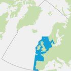
Area Assessed
Printable Summary
Background
OSPAR’s strategic objective with regard to eutrophication is to combat eutrophication in the OSPAR Maritime Area, with the ultimate aim to achieve and maintain a healthy marine environment where anthropogenic eutrophication does not occur. Dissolved oxygen is one of a suite of five eutrophication indicators. When assessed and considered together in the OSPAR Common Procedure in a multi-step method, the suite can be used to diagnose eutrophication.
Excessive enrichment of marine water with nutrients may lead to algal (phytoplankton) blooms, with the possible consequence of undesirable disturbance to the balance of organisms in the marine ecosystem and overall water quality. Undesirable disturbance includes shifts in the composition and extent of flora and fauna and depletion of oxygen caused by decomposition of accumulated organic material produced by phytoplankton or seaweed communities during their growing seasons. Oxygen depletion may result in behavioural changes or death of fish and other species. Although oxygen depletion can be an indirect effect of nutrient enrichment, other pressures often complicate the identification of causal links between disturbances and nutrient enrichment. Factors that influence oxygen concentrations include changes in water temperature and salinity and climate change. Seasonal oxygen depletion can be a natural localised process, particularly where the water column stratifies seasonally.
Oxygen concentrations above 6 mg/l are considered to support marine life with minimal problems, while concentrations less than 2 mg/l (hypoxia, i.e. oxygen deficiency) (Figure 1) are considered to cause severe problems.
Observations from the Baltic Sea show that when the oxygen content in the bottom water is very low, the only organisms that are able to thrive are the bacteria that live on and in the seafloor (Figure 2).
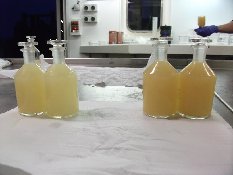
Figure 1: Water samples collected from the Celtic Seas during a Karenia mikimotoi bloom (July 2011). Surface samples were darker (higher concentrations of dissolved oxygen) than near-bottom samples (lower dissolved oxygen). © Elisa Capuzzo, Cefas
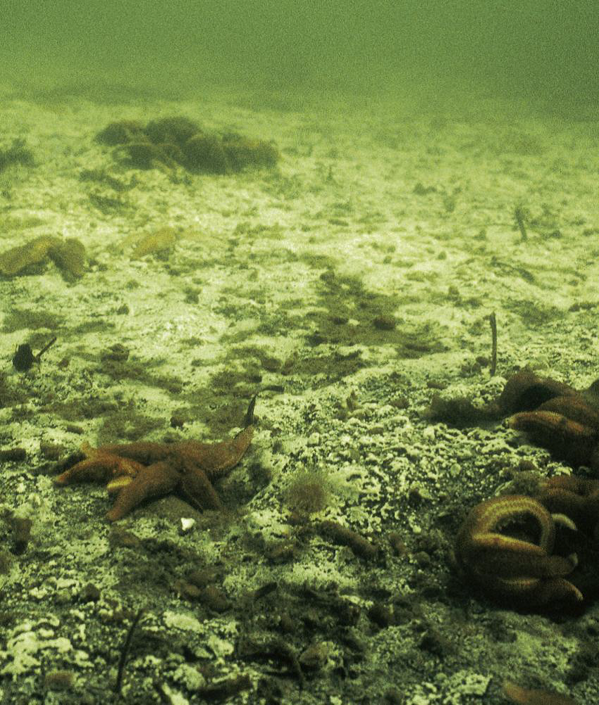
Figure 2: Low oxygen conditions in the Baltic Sea. The patches of white sulphur bacteria form a shroud © Peter Bondo Christensen
Eutrophication is the result of excessive enrichment of water with nutrients. This may cause accelerated growth of algae and / or higher forms of plant life (Council Directive 91/676/EEC). This may result in an undesirable disturbance to the balance of organisms present and thus to the overall water quality. Undesirable disturbances can include shifts in the composition and extent of flora and fauna and the depletion of oxygen due to decomposition of accumulated biomass. Such disturbances then have other effects, such as changes in habitats and biodiversity, blooms of nuisance algae or macroalgae, decrease in water clarity and behavioural changes or even death of fish and other species. Identifying causal links between these disturbances and nutrient enrichment can be complicated by other pressures. Cumulative effects, including climate change, may have similar effects on biological communities and dissolved oxygen, further complicating efforts to demonstrate causal links.
The OSPAR Commission’s strategic objective, with regard to eutrophication, is to combat eutrophication in the OSPAR Maritime Area, with the ultimate aim that by 2020 the OSPAR Maritime Area is a healthy marine environment where anthropogenic eutrophication does not occur (OSPAR Agreement 2010-3). The OSPAR Eutrophication Strategy requires assessment of eutrophication to be based on the ecological consequences of nutrient enrichment and not just on nutrient enrichment alone, i.e. finding reliable evidence for accelerated growth of algae and / or macrophytes caused by anthropogenic nutrient enrichment, leading to undesirable disturbance. Eutrophication is diagnosed using OSPAR’s harmonised criteria of nutrient inputs, concentrations and ratios, chlorophyll-a concentrations, phytoplankton indicator species, macrophytes, dissolved oxygen levels, incidence of fish kills and changes in zoobenthos (OSPAR Agreement 2010-8). As there is no single indicator of disturbance caused by marine eutrophication, OSPAR applies a multi-step method using the harmonised criteria. Eutrophication is considered to have occurred if there is evidence for all of the stages shown in Figure a and of causal links between them (ECJ, 2009).
For OSPAR’s Intermediate Assessment 2017, five harmonised eutrophication criteria have been assessed at a regional scale: nutrient inputs, nutrient concentrations and ratios, chlorophyll-a concentrations, concentrations of the nuisance algae Phaeocystis, and dissolved oxygen levels. These are highlighted in Figure a. The individual assessment results of any one of these five common indicators do not diagnose eutrophication by themselves. However, the assessments provide useful information about trends and are important for informing management measures.
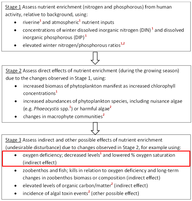
Figure a: Three stages in the identification of eutrophication. The criteria marked ¹ are common indicators for the OSPAR Intermediate Assessment 2017. The criteria marked ² are not relevant in all countries’ waters. The common indicator assessed here (dissolved oxygen levels) is outlined in red
The concentration of dissolved oxygen was assessed as an indicator of indirect effects of nutrient enrichment (Figure a). Depletion of oxygen may be caused by decomposition of accumulated organic material produced by algae (phytoplankton) or seaweed communities during their growing seasons, and may result in behavioural changes or death of fish and other species. However, oxygen depletion is not necessarily a consequence of nutrient enrichment and may be influenced by several other factors, including changes in water temperature and salinity. Seasonal oxygen depletion can be a natural localised process, particularly where the water column stratifies seasonally.
Available data were used to calculate the mean concentration and percentage saturation of dissolved oxygen in the lowest quartile (25%) of the data within 10 m of the seafloor in marine waters (salinity ≥30) during the stratification season (1 July–31 October).
Dissolved oxygen was assessed in the OSPAR Quality Status Report (QSR) 2010 as part of the Common Procedure for the identification of eutrophication. There is no comparable regional indicator assessment of dissolved oxygen.
Near seafloor oxygen concentrations >6 mg/l are considered to cause minimal problems to marine life (Best et al., 2007), while concentrations <2 mg/l (hypoxia) are considered to cause severe problems (Levin et al., 2009). Assessment levels used by OSPAR countries applying the Common Procedure (OSPAR 2013-8) range from 2 to 6 mg/l, and are applied over specified assessment periods. For the third application of the Common Procedure , this period is 2006–2014. However, for trend assessments, data from longer time series are used, where available. Data from the period 1990–2014 were used to assess trends in the data.
OSPAR IA 2017 Indicator Assessment values are not to be considered as equivalent to proposed European Union Marine Strategy Framework Directive (MSFD) criteria threshold values, however they can be used for the purposes of their MSFD obligations by those countries that wish to do so.
Data
Data on dissolved oxygen concentrations for the period 1990–2014 and all supporting information (e.g. latitude, longitude, water column depth, sample depth, temperature, salinity) were obtained from ICES[1], (Figure b)[2]. Data were filtered for the assessment, to obtain data from near the seafloor[3] in marine waters (i.e. coastal and offshore waters with salinity ≥30, see OSPAR Agreement 2013-8) during the stratification season (1 July–31 October)[4]. For the Skagerrak and Kattegat, data from fjords were filtered to exclude high salinity bottom waters. Percentage saturation of dissolved oxygen was calculated from oxygen concentrations, temperature and salinity.
Spatial scales
Two scales of data aggregation were adopted for the assessment, the large-scale common assessment areas, and smaller ICES rectangles. The large-scale common assessment areas were the Greater North Sea (northern North Sea; southern North Sea; the English Channel; the Skagerrak; the Kattegat; and the Sound), the Celtic Seas, and the Bay of Biscay and Iberian Coast. The smaller scale of rectangles (1° Longitude by 0.5° Latitude) helps to identify localised areas that may be characterised by low oxygen levels (‘hotspots’). In the south-eastern part of the North Sea, data were analysed by individual rectangles and in an aggregated dataset, due to limited data in many individual rectangles.
The outcome per area was summarised in a map showing the mean dissolved oxygen concentrations in four ranges (<2, 2–4, 4–6 and >6 mg/l) for the period 1 July to 31 October in 2014.
Trend Assessments
For the full time series (1990–2014), means in the lowest quartile of the data per stratification season per year were used to identify trends in the data. Where fewer than five data points were available in any given year in an assessment area, these data points were excluded, in order to avoid bias in the analysis.
Trends were assessed using the Mann-Kendall non-parametric test for trend analysis (Mann, 1945; Kendall, 1975). The R library package ‘emon’ was used (Barry and Maxwell, 2015). Where p<0.05, it was assumed that there was a significant trend. Where p>0.05, a trend could not be detected statistically. Where trends were significant, weighted least squares (WLS) regression lines were calculated, using the 95% confidence intervals for the means.
COMP3 Assessment Period
For the period relevant to the third application of the Common Procedure (2006–2014), data on oxygen concentrations were analysed by the large-scale common assessment areas and by ICES rectangles (individual and aggregated). Mean oxygen concentrations in the lowest quartile of the data per area were summarised in maps using four data ranges (<2, 2–4, 4–6 and >6 mg/l). For the large-scale common assessment regions, there were sufficient data per region to map the results.
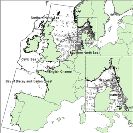
Figure b: Assessed area showing sites where ICES data were available for the period 1990–2014. Filtered by season (stratification season 1 July–31 October), depth (within 10 m of the seafloor) and salinity (≥30) to obtain the specific data required for the assessments. Data from fjords were filtered to exclude high salinity bottom waters
[1][1]Datasets were requested from ICES in May 2015 and updated in December 2016, from: 35N to 63N, 13W to 16E (to encompass OSPAR Maritime Area “Greater North Sea”, “Celtic Seas” and “Bay of Biscay and Iberian Coast”). 1/1/1990 to present, temperature, salinity and oxygen concentration. This comprised CTD profiles, reduced to standard depths (0m, 5m, 10m, 15, 20, 25, 30, 35, 40, 45, 50, 55, 60, 65, 70, 75, 80, 85, 90, 95, 100, 120, 140, 160, 180, 200, 225, 250, 275, 300, 325, 350, 375, 400, 425, 450, 475, 500, 525, 550, 575, 600, 625, 650, 675, 700, 725, 750, 775, 800, 850, 900, 950, 1000, 1100, 1200, 1300, 1400, 1500, 1600, 1700, 1800, 1900, 2000, 2200, 2400, 2500, 2600, 2800, 3000, 3200, 3400, 3600, 3800, 4000, 4500, 5000, 6000, 6500, 7000, 8000m, etc, with deepest measurement always retained) and bottle data samples. Data from France were not in the ICES database and were provided separately.
[2] For the UK, this does not include data collected under the Water Framework Directive (WFD).
[3] Data were filtered to select data within 10m of the seafloor, and then the deepest sample was selected for the analyses; where the water column was deeper than 500 m, the data were not included in the analyses.
[4] Number of data points available after application of filters. In brackets = 1990-2014; in bold = 2006-2014: northern North Sea, NNS (735) 271; southern North Sea, SNS (1505) 422; Skagerrak (1775) 400; Kattegat (2417) 688; The Sound (426) 125; English Channel (2256) 1273; Celtic Sea (2851) 2669; Bay of Biscay and Iberian Coast (1515) 1403.
Results
Mean near-bed dissolved oxygen concentrations (2006–2014) assessed in large-scale regions of the northern North Sea, southern North Sea, English Channel, Celtic Seas, and Bay of Biscay and Iberian Coast were >6 mg/l. Mean near-bed oxygen concentrations were lower in the Skagerrak (5.25 mg/l), Kattegat (3.98 mg/l) and the Sound (2.80 mg/l). Oxygen concentrations in these three regions are strongly influenced by local eco-hydrodynamic conditions.
No statistically significant temporal trends were observed (1990–2014) in near-bed oxygen concentrations or percentage saturation in most of the large-scale regions (northern North Sea, southern North Sea, Skagerrak, Sound, English Channel, Celtic Seas, and Bay of Biscay and Iberian Coast). The Kattegat was the only exception, with significant upward trends observed in oxygen concentrations and percentage saturation.
Within the large-scale regions, available data (1990–2014) were analysed at a smaller scale using ICES rectangles. Analyses showed that mean near-bed oxygen concentrations in the lowest quartile of the data during the summer stratification season were >6 mg/l in most ICES rectangles in each region, except in the southern North Sea and the Kattegat (Figure 3). For the southern North Sea, rectangles with mean values of <6 mg/l indicate localised areas with lower oxygen concentrations. These rectangles are mostly located in the eastern southern North Sea (outlined in bold in Figure 3), a region with a high degree of hydrodynamic variability. No temporal trends were identified in 12 of the 13 individual rectangles in the eastern southern North Sea (i.e. dissolved oxygen concentrations showed no change). A significant downward trend was observed in one rectangle (in the Skagerrak off the southeast coast of Norway). When all the data in these rectangles were aggregated (Figure 3) into one dataset, no statistically significant trend was found at the large scale.
In the Skagerrak and Kattegat, ICES rectangles also showed mean near-bed oxygen concentrations of <6 mg/l. However, the specific regional characteristics of this area mean that these levels are not considered to indicate oxygen deficiency. For the Kattegat, analyses of rectangles indicate areas with higher mean near-bed concentrations (4–6 mg/l) than those calculated using the large-scale regional analysis (2–4 mg/l).
In the Bay of Biscay and Iberian Coast, four rectangles showed lower oxygen concentrations (4–6 mg/l) but there were insufficient data for detailed analyses. One rectangle in the Celtic Seas showed a mean near-bed oxygen concentration (5.8 mg/l) towards the upper end of the 4–6 mg/l range, indicating a localised area with low oxygen.
Overall, results indicate that oxygen concentrations, when analysed at larger scales, were not depleted during the shorter (2006–2014) and longer (1990–2014) assessment periods.
Confidence ratings in terms of data availability and methodology used are moderate.
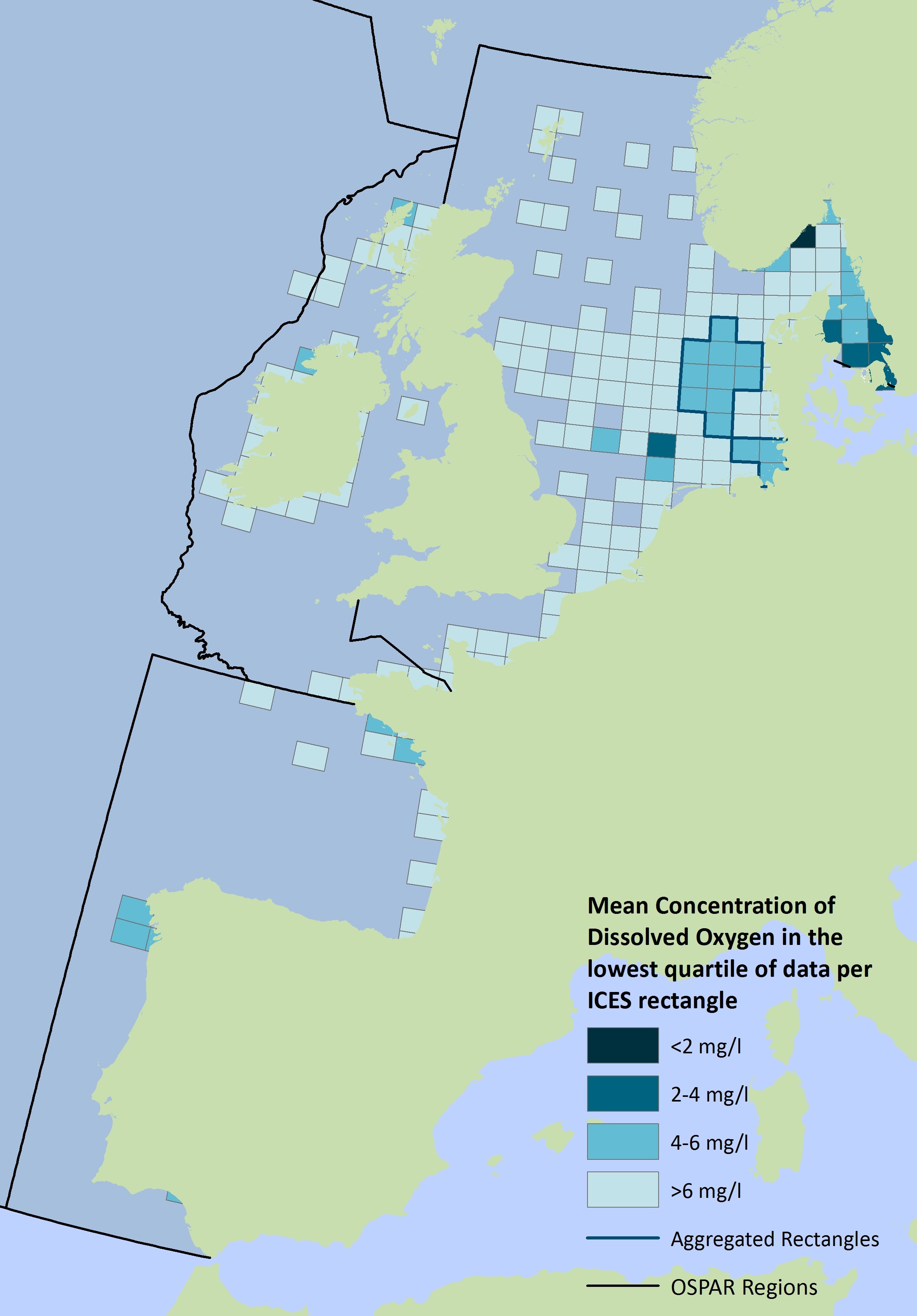
Figure 3: Mean concentration of dissolved oxygen in the lowest quartile of the data plotted by ICES rectangles for the period 1990–2014. Rectangles aggregated for analyses are outlined in bold. Data were filtered by season (stratification season 1 July–31 October), depth (within 10 m of the seafloor), and salinity (≥30). Results are shown for rectangles where there were five or more data points. Blank areas indicate where there were no data or insufficient data
For temporal trend analyses, longer-term datasets (1990–2014) were used. Mann Kendall analyses were considered to provide a robust estimate of significant trends. Downward trends indicate that oxygen levels are decreasing over time and may be a cause for concern. Where Mann Kendall analyses showed significant trends, weighted linear (least squares) regression lines were used to show the trends in oxygen concentration and percentage saturation.
Analyses of longer-term data in the Greater North Sea, Celtic Seas, and Bay of Biscay and Iberian Coast regions showed that oxygen concentrations (1990–2014) varied from year to year in each of the assessment areas. Analyses by ICES rectangles showed similar interannual variability in the data.
For the period 2006–2014, far fewer ICES rectangles had sufficient data (>5 data points) for an overall assessment (Figure c). In the northern North Sea and southern North Sea, five rectangles had mean values of <6 mg/l (compared to 16 using the 1990–2014 time series). In the Skagerrak and Kattegat, approximately half of rectangles had mean values <6 mg/l.
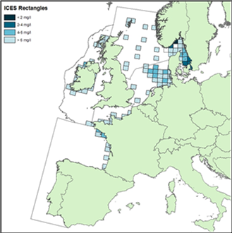
Figure c: Mean concentration of dissolved oxygen in the lowest quartile of the data plotted by ICES rectangles for the period 2006–2014. Results are shown for rectangles where there were five or more data points, after filtering by season (stratification season 1 July–31 October), depth (within 10 m of the seafloor) and salinity (≥30) to obtain the specific data required for the assessments. Blank areas indicate where there were no data or insufficient data
Northern North Sea and southern North Sea
For the large-scale regions of the northern North Sea and southern North Sea, mean near-bed dissolved oxygen concentrations for 2006–2014 were >6 mg/l. Stratified-season means in the lowest quartile were >6 mg/l and ≥60% saturation in all years in the northern North Sea, and above 5 mg/l and ≥60% saturation in all years in the southern North Sea (Figure d). In both the northern North Sea and southern North Sea, 95% confidence levels indicate high confidence in the data. Mann-Kendall analyses using the annual mean data showed no significant trends in oxygen concentration and percentage saturation of dissolved oxygen (Table a and Table b).
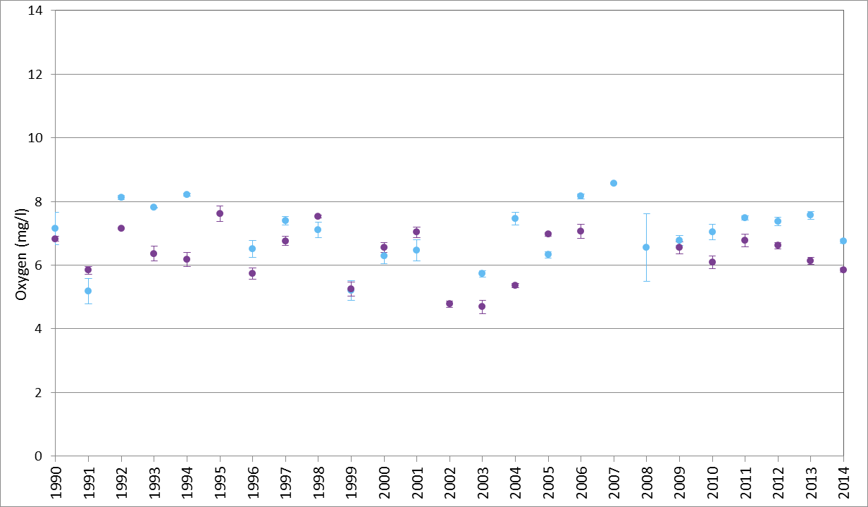
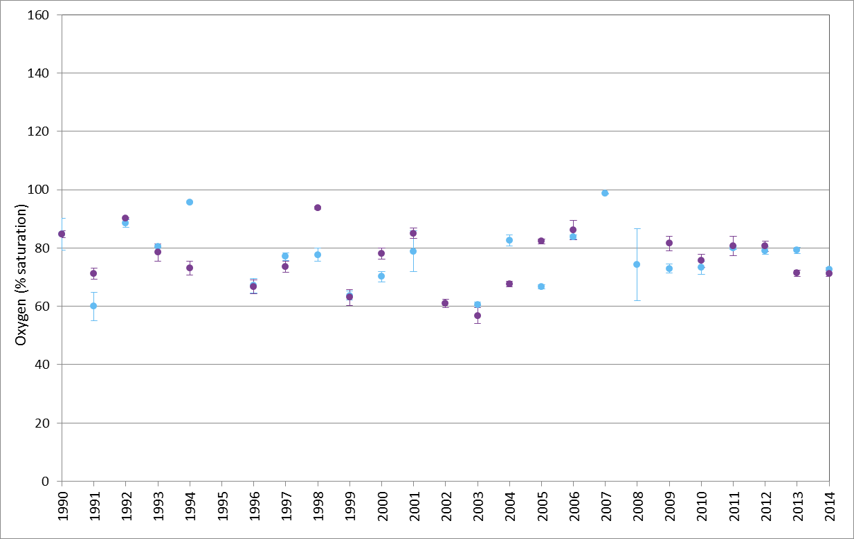
Figure d: Dissolved oxygen in the southern North Sea (purple dots) and northern North Sea (blue dots) for the period 1990–2014, shown as stratified-season (1 July–31 October) means for the lowest quartile of the data ± the 95% confidence interval. Results are shown for years with five or more data points after filtering by season, depth (within 10 m of the seafloor) and salinity (≥30) (for additional details on number of samples per year and minimum values, see Table e). (i) oxygen concentration (mg/l), (ii) oxygen percentage saturation
Within the southern North Sea, ICES rectangles with mean dissolved oxygen values of <6 mg/l in the lowest quartile of the data were observed mainly in the eastern areas (outlined in bold in Figure e), and indicate localised areas (‘hotspots’) with lower oxygen levels (mean 4–6 mg/l, Figure 3 and Figure e; minimum = 2.8 mg/l, Table d). These results broadly agree with previous findings (e.g. Topcu and Brockmann, 2015; Große et al., 2016), although the ICES dataset did not include the earlier data (1980–1990) and local datasets used in those previous studies. The hotspots are located in regions that show a high degree of hydrodynamic variability. Most are relatively shallow (less than about 40 m), with competing influences from riverine outflow (such as the Elbe), wind mixing (e.g. in shallow areas along the Danish coast), and localised influences such as in the Elbe channel where seasonal stratification occurs in warm years and low oxygen conditions may occur near the bed if there is low through-flow (van Leeuwen et al., 2015).
Several researchers have shown that water column stratification represents a major process regulating the seasonal dynamics of bottom oxygen levels (e.g. Topcu and Brockmann, 2015; Queste et al., 2016). However, it has been shown that the lowest oxygen conditions in the North Sea do not occur in the areas of strongest stratification (e.g. Große et al., 2016; Queste et al., 2016). Although stratification is an important prerequisite for oxygen deficiency, the changes observed represent the end result of a complex interaction between hydrodynamic and biological processes. Oxygen consumption may be affected by biological processes such as pelagic and benthic remineralisation of organic matter, zooplankton respiration, nitrification and denitrification. Große et al. (2016) analysed oxygen dynamics under stratified conditions in the southern North Sea. They found that biological consumption processes (mainly by bacteria) control the sub-thermocline oxygen conditions. There is a strong link between near-surface primary production and the export of organic matter into the bottom water layer, enhancing bacterial remineralisation. These processes in combination with the size of the sub-thermocline water volume, control the evolution of the oxygen concentration. Regions with high surface net primary production and a small sub-thermocline volume are particularly susceptible to oxygen deficiency.
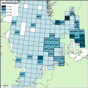
Figure e: ICES codes for rectangles in the northern North Sea, southern North Sea, Skagerrak and Kattegat where mean near-bed oxygen concentrations in the lowest quartile of available data (1990–2014) were <6 mg/l, after filtering by stratified-season (1 July–31 October), depth (within 10 m of the seafloor) and salinity (≥30). For the eastern part of the southern North Sea, data were analysed by rectangle for long-term trends, and using aggregated data from all adjoining rectangles (outlined in bold)
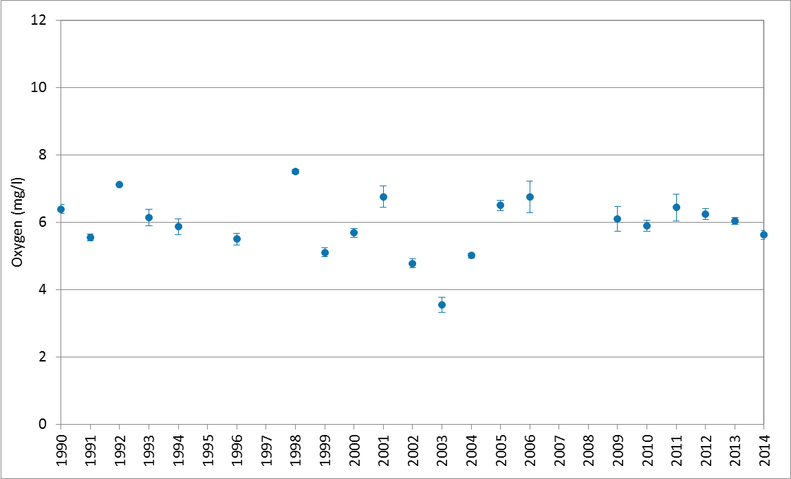
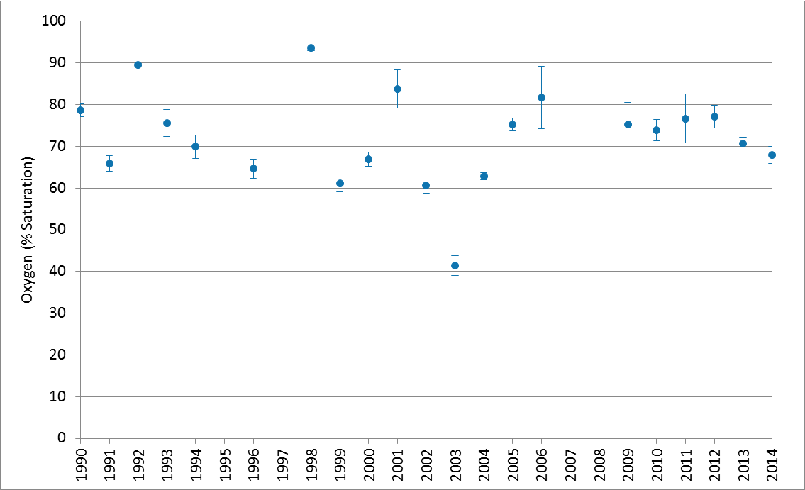
Figure f: Dissolved oxygen (1990–2014) in aggregated ICES rectangles in the eastern part of the southern North Sea with mean concentrations <6 mg/l (see Figure 3). Data are shown as stratified-season (1 July–31 October) means in the lowest quartile of the data ± the 95% confidence interval. Results are shown for years with five or more data points after filtering by season, depth (within 10 m of the seafloor) and salinity (≥30). (i) oxygen concentration (mg/l), (ii) oxygen percentage saturation
Mann Kendall analyses indicated no significant trends in dissolved oxygen concentration or saturation in 12 of the 13 ICES rectangles or in the aggregated dataset for the south-eastern part of the North Sea (Figure f). ICES rectangle 40F7 was found to have a significant downward trend in dissolved oxygen concentration (Table c). Summary statistics for the aggregated dataset (Table d) indicate variability in the data, with measurements ranging from a minimum of 2.82 mg/l to a maximum of 12 mg/l, and mean values in the lowest quartile of the data of 3.55–7.5 mg/l in years when more than four data points were available.
| Region | n | MK Statistic | p-value |
|---|---|---|---|
| Bay of Biscay and Iberian Coast | 14 | 25 | 0.193 |
| Celtic Sea | 17 | 5 | 0.881 |
| English Channel | 12 | -4 | 0.842 |
| Kattegat | 25 | 106 | 0.0135 |
| Northern North Sea | 23 | -1 | 1 |
| Skagerrak | 25 | -66 | 0.131 |
| Southern North Sea | 24 | -20 | 0.641 |
| The Sound | 25 | 66 | 0.129 |
Data filtered by season, depth (within 10 m of the seafloor) and salinity (≥30). The sign of the MK statistic gives the direction of the trend. Statistically significant trend (p<0.05) in bold. n, number of data points (years).
| Region | n | MK statistic | p-value |
|---|---|---|---|
| Bay of Biscay and Iberian Coast | 15 | 33 | 0.114 |
| Celtic Seas | 18 | -23 | 0.489 |
| English Channel | 15 | 5 | 0.847 |
| Kattegat | 25 | 110 | 0.010 |
| Northern North Sea | 23 | 9 | 0.834 |
| Skagerrak | 25 | -68 | 0.119 |
| Southern North Sea | 24 | -20 | 0.640 |
| The Sound | 25 | 66 | 0.129 |
Data filtered by season, depth (within 10 m of the seafloor) and salinity (≥30). The sign of the MK statistic gives the direction of the trend. Statistically significant trend (p<0.05) in bold. n, number of data points (years)
| Region | n | MK statistic | p-value |
|---|---|---|---|
| esNS | 23 | -0.496 | 0.620 |
| ICES 36F8 | 15 | 0.741 | 0.458 |
| ICES 37F7 | 19 | 0.280 | 0.780 |
| ICES 37F8 | 20 | -0.130 | 0.897 |
| ICES 38F6 | 21 | 0.151 | 0.880 |
| ICES 39F5 | 19 | -0.490 | 0.6242 |
| ICES 39F6 | 19 | 0.910 | 0.363 |
| ICES 40F5 | 8 | -1.861 | 0.063 |
| ICES 40F6 | 7 | 0 | 1 |
| ICES 40F7 | 11 | -2.024 | 0.043 |
| ICES 41F5 | 7 | -0.302 | 0.763 |
| ICES 41F6 | 9 | -1.037 | 0.3 |
| ICES 41F7 | 10 | 1.073 | 0.283 |
| ICES 42F6 | 11 | -1.09 | 0.276 |
Using stratified-season (1 July–31 October) means in the lowest quartile of data filtered by season, depth (within 10 m of the seafloor) and salinity (≥30). Data were also analysed using aggregated data from all adjoining rectangles (see esNS – eastern southern North Sea). The sign of the MK statistic gives the direction of the trend. Statistically significant trend (p<0.05) in bold. n, number of years with data. Data from all years were used in analyses, including years when the number of data points (count) was less than five (see Table d)
| Year | Count | Min Value | Max Value | Median | Mean | SD | SE | meanQ25 | sdQ25 |
|---|---|---|---|---|---|---|---|---|---|
| 1990 | 58 | 5,16 | 9,70 | 7,30 | 7,28 | 0,74 | 0,10 | 6,39 | 0,51 |
| 1991 | 31 | 5,20 | 9,20 | 6,63 | 6,78 | 1,07 | 0,19 | 5,55 | 0,28 |
| 1992 | 20 | 7,06 | 8,33 | 7,39 | 7,52 | 0,43 | 0,10 | 7,12 | 0,04 |
| 1993 | 18 | 5,67 | 8,70 | 7,51 | 7,26 | 0,84 | 0,20 | 6,14 | 0,50 |
| 1994 | 19 | 5,17 | 8,35 | 7,02 | 7,01 | 0,90 | 0,21 | 5,86 | 0,51 |
| 1995 | 1 | 7,80 | 7,80 | 7,80 | 7,80 | NA | NA | 7,80 | NA |
| 1996 | 25 | 5,03 | 8,65 | 6,49 | 6,45 | 0,83 | 0,17 | 5,50 | 0,42 |
| 1997 | 1 | 6,72 | 6,72 | 6,72 | 6,72 | NA | NA | 6,72 | NA |
| 1998 | 37 | 7,25 | 8,56 | 8,05 | 7,97 | 0,34 | 0,06 | 7,50 | 0,21 |
| 1999 | 18 | 4,67 | 7,52 | 5,92 | 5,97 | 0,73 | 0,17 | 5,10 | 0,27 |
| 2000 | 29 | 5,12 | 8,15 | 7,05 | 6,86 | 0,88 | 0,16 | 5,68 | 0,33 |
| 2001 | 14 | 5,99 | 8,16 | 7,45 | 7,36 | 0,52 | 0,14 | 6,76 | 0,54 |
| 2002 | 41 | 3,93 | 7,33 | 6,16 | 5,90 | 0,86 | 0,13 | 4,78 | 0,42 |
| 2003 | 26 | 2,82 | 8,62 | 5,72 | 5,92 | 1,97 | 0,39 | 3,55 | 0,56 |
| 2004 | 66 | 4,50 | 9,86 | 6,07 | 6,31 | 1,18 | 0,15 | 5,01 | 0,28 |
| 2005 | 28 | 6,00 | 8,86 | 7,59 | 7,57 | 0,81 | 0,15 | 6,49 | 0,41 |
| 2006 | 24 | 4,57 | 12,00 | 7,86 | 7,90 | 1,38 | 0,28 | 6,75 | 1,11 |
| 2009 | 14 | 5,33 | 7,62 | 6,85 | 6,83 | 0,62 | 0,17 | 6,10 | 0,62 |
| 2010 | 15 | 5,70 | 7,60 | 6,97 | 6,77 | 0,67 | 0,17 | 5,89 | 0,30 |
| 2011 | 21 | 5,23 | 8,50 | 7,52 | 7,33 | 0,78 | 0,17 | 6,43 | 0,89 |
| 2012 | 19 | 5,86 | 7,96 | 6,93 | 6,94 | 0,55 | 0,13 | 6,24 | 0,33 |
| 2013 | 17 | 5,70 | 7,59 | 6,52 | 6,58 | 0,49 | 0,12 | 6,03 | 0,19 |
| 2014 | 36 | 5,00 | 7,92 | 6,12 | 6,37 | 0,68 | 0,11 | 5,63 | 0,39 |
| ALL | 578 | 2,82 | 12,00 | 7,05 | 6,86 | 1,11 | 0,05 | 5,40 | 0,64 |
Skagerrak
In the Skagerrak, mean near-bed dissolved oxygen concentrations in the lowest quartile (2006–2014) over the large-scale assessment region were 4–6 mg/l. Annual means were generally above 3–4 mg/l and 30–40% saturation (Figure g). Variability in the data was high and is largely attributable to the complex oceanography of the region, and high environmental variability (Erlandsson et al., 2006; Hansen and Bendsten, 2013a,b; Lehmann et al., 2014). The Skagerrak is well known for having strong haline stratification (van Leeuwen et al., 2015). Water depths reach 200 m close to the coast, and the environmental conditions that lead to oxygen deficiency in the Skagerrak are different to those influencing the eastern part of the southern North Sea and the Kattegat. The deep water is open and well ventilated horizontally, resulting in oxygen deficiency being largely restricted to fjords, which were not included in this assessment (SMHI, 2016).
Mann-Kendall analyses using the annual mean data showed no significant trends in oxygen concentration or percentage saturation in the Skagerrak (Table a and Table b).
Analyses by ICES rectangle showed that regions with lower oxygen concentrations (i.e. <6 mg/l) were located in coastal regions. However, these values are not considered to indicate oxygen deficiency in this region.
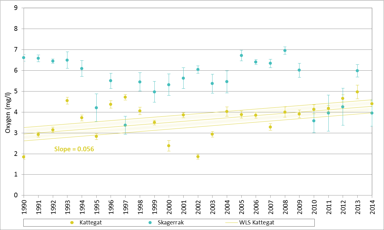
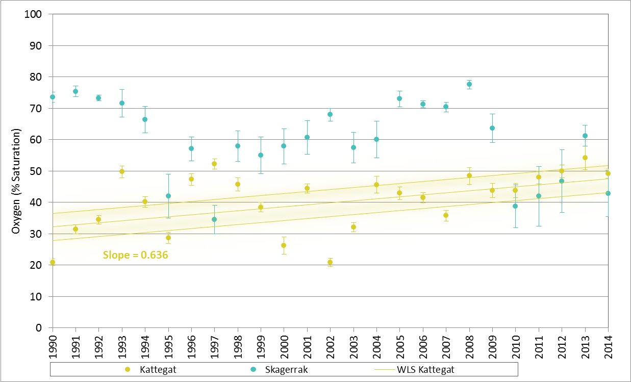
Figure g: Dissolved oxygen in the Kattegat (yellow dots) and Skagerrak (blue dots) for the period 1990–2014, shown as stratified-season (1 July–31 October) means for the lowest quartile of the data ± the 95% confidence interval. Results are shown for years with five or more data points after filtering by season, depth (within 10 m of the seafloor) and salinity (≥30) (for additional details on number of samples per year and minimum values, see Table e). (i) oxygen concentration (mg/l), (ii) oxygen percentage saturation. WLS, weighted least squares regression using the confidence interval as weight. Shading indicates 95% confidence levels around the WLS. The slope of the WLS regression is shown; significant trends were identified using Mann-Kendall analyses
Kattegat
For the period 2006–2014, annual stratified-season means in dissolved oxygen concentration were lower than for the other assessment areas of the Greater North Sea, but generally above 2 mg/l and 20% saturation (Figure g). Analyses by ICES rectangle showed that regions with the lowest oxygen concentration (2–4 mg/l) were located in the southern parts of the Kattegat. These values are not considered to indicate oxygeHeading 3n deficiency in this region. Variability in the data was high due to complex topography and oceanography (Hansen and Bendsten, 2013a,b; Lehmann et al., 2014; SMHI, 2016). The Kattegat and Sound are particularly vulnerable to hypoxia and anoxia (absence of oxygen or severe oxygen depletion), because the halocline is strong and tends to lie at 15–30 m depth. In some areas, the halocline may at times be near the seafloor. During these events, the volume of bottom water is low and oxygen levels depend on replenishment by horizontal advection.
For the offshore Kattegat, 2002 was a particularly hypoxic year (i.e. <2 mg/l, Figure g). This was attributed to several weeks of extremely calm weather, which prevented the horizontal advection of oxygen across the seafloor (Ærtebjerg et al., 2002; SMHI, 2007).
Mann-Kendall analyses showed a significant upward trend in the Kattegat for dissolved oxygen concentration (Table a) and percentage saturation (Table b).
The Sound
Annual stratified-season means in dissolved oxygen concentration (Figure h) were highly variable, ranging from 1 to 5 mg/l and 10% to 55% saturation during the period 2006–2014. Variability in the data was high due to complex topography and oceanography (Hansen and Bendsten 2013a,b; Lehmann et al., 2014; SMHI 2016). Mann-Kendall analyses using the annual mean data showed no significant trends in oxygen concentration or percentage saturation (Tables a and b).
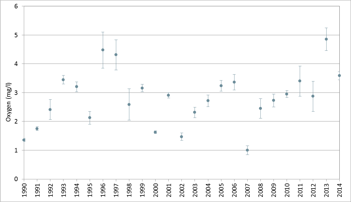
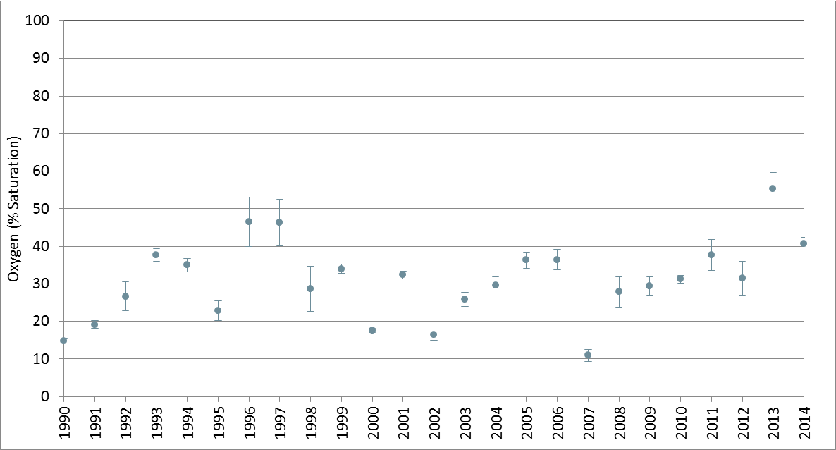
Figure h: Dissolved oxygen in the Sound for the period 1990–2014, shown as stratified-season (1 July–31 October) means for the lowest quartile of the data ± the 95% confidence interval. Results are shown for years with five or more data points after filtering by season, depth (within 10 m of the seafloor) and salinity (≥30) (for additional details on number of samples per year and minimum values, see Table e). (i) oxygen concentration (mg/l), (ii) oxygen percentage saturation
English Channel
In the English Channel, mean near-bed dissolved oxygen concentrations in the lowest quartile of the data were >6 mg/l. Annual stratified-season means (Figure i) were generally >6 mg/l and 80% saturation, with relatively few data points in this area.
The Mann-Kendall analyses using the annual mean data showed no significant trends in oxygen concentration or percentage saturation in the English Channel (Tables a and b).
Celtic Seas
The mean near-bed dissolved oxygen concentration (2006–2014) in the lowest quartile of the data in the large-scale region of the Celtic Seas was >6 mg/l. Annual stratified-season means (Figure i) were generally >6 mg/l and 80% saturation, with relatively few data points in this area.
In one ICES rectangle (38E1) in the Celtic Seas, the mean near-bed oxygen concentration in the lowest quartile of the data was in the 4–6 mg/l range. Data in this rectangle are available from 2007 only, and the mean value in the lowest quartile of the data (5.8 mg/l) is the same in both the longer dataset (1990–2014) and the shorter dataset (2006–2014). Oxygen deficiency in this region is attributable to local issues within Killybegs Harbour, as reported on in the third application of the Common Procedure (see EPA and Marine Institute, 2016).
The Mann-Kendall analyses using the annual mean data showed no significant trends in oxygen concentration or percentage saturation in the Celtic Seas (Tables a and b).
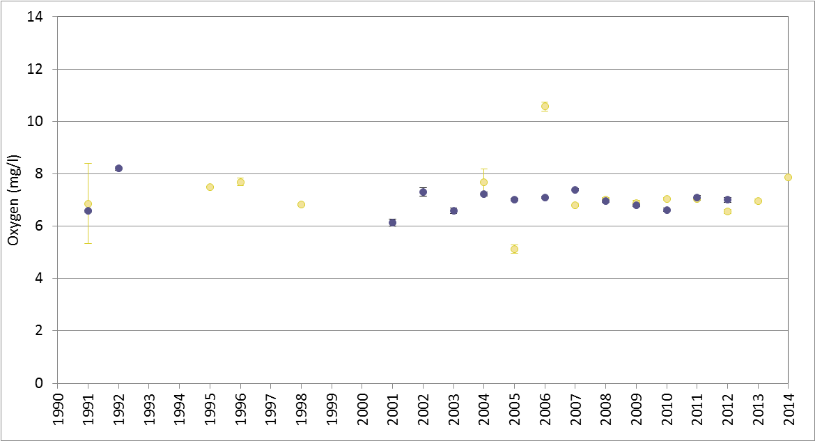
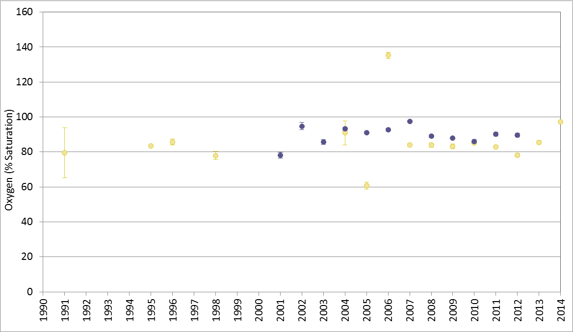
Figure i: Dissolved oxygen in the English Channel (purple dots) and Celtic Seas (yellow dots) for the period 1990–2014, shown as stratified-season (1 July–31 October) means for the lowest quartile of the data ± the 95% confidence interval. Results are shown for years with five or more data points after filtering by season, depth (within 10 m of the seafloor) and salinity (≥30) (for additional details on number of samples per year and minimum values, see Table e). (i) oxygen concentration (mg/l), (ii) oxygen percentage saturation.
Bay of Biscay and Iberian Coast
For the large-scale assessment region for the Bay of Biscay and Iberian Coast, mean near-bed dissolved oxygen concentrations for the period 2006–2014 were >6 mg/l. Data availability was poor in this region. Four ICES rectangles indicated lower oxygen concentrations (4–6 mg/l, Figure 3) but there were insufficient data for detailed analyses. Mann-Kendall analyses showed no significant trends in oxygen concentration or percentage saturation for the Bay of Biscay and Iberian Coast region.
Confidence ratings
Confidence in data availability is moderate-to-high due to temporal and / or spatial gaps in the data in many regions. The ICES database includes a large amount of data on dissolved oxygen, measured from all depths. Once these data were filtered by depth, season and salinity, the dataset was considerably reduced: from approximately 860 000 data points, including binned CTD data, to approximately 14 000 data points for the period 1990–2014, and approximately 7300 data points for the period 2006–2014. The largest dataset (see Table e) was available for the Celtic Seas; most data (2669 data points) were collected from coastal regions (Figure b) from 2006 onwards (Table e), indicating gaps in spatial and temporal coverage. Large datasets were also available for the English Channel (2256 data points) and Iberian Coast and Bay of Biscay (1515 data points), but they also represented largely coastal sampling (Figure b) from 2001 onwards (Table e), also indicating gaps in space and time. Confidence ratings for data availability are therefore moderate in these regions. Confidence ratings are higher for the Kattegat, Skagerrak and southern North Sea. Relatively large datasets were available in these regions (Kattegat 2417 data points, Skagerrak 1775 data points, southern North Sea 1505 data points, Table e); spatial coverage appeared to be sufficient (Figure b) and data were collected fairly consistently from 1990 (Table e), giving greater confidence in assessment outcomes. For the Kattegat and Skagerrak, this may be outweighed by issues relating to complex oceanography in these areas. The available dataset in the northern North Sea was relatively small (735 data points, Table e), although temporal and spatial coverage appeared to be sufficient for this region, which is not known to have low oxygen levels. Confidence ratings are therefore also high for this region.
Confidence in the methods used for assessing oxygen deficiency is moderate overall. The approach has been developed over many years, and applied in published international assessments. In this assessment, however, the method has been refined to focus specifically on measurements from near the seafloor, and to use the mean of the lowest quartile of the data, rather than the 5th percentile of all data, which has been used in previous assessments. The methodology requires further development to address questions about the feasibility and practicalities of near-seafloor monitoring and assessment.
| None | Iberian and Bay | Celtic Seas | English Channel | Kattegat | Northern North | Skagerrak | Southern North | Sound | ||||||||||||||||
|---|---|---|---|---|---|---|---|---|---|---|---|---|---|---|---|---|---|---|---|---|---|---|---|---|
| Year | n | min | mean Q25 | n | min | mean Q25 | n | min | mean Q25 | n | min | mean Q25 | n | min | mean Q25 | n | min | mean Q25 | n | min | mean Q25 | n | min | mean Q25 |
| 1990 | 12 | 4.02 | 4.88 | 4 | 7.53 | 7.53 | 4 | 6.70 | 6.70 | 123 | 0.79 | 1.84 | 12 | 6.30 | 7.15 | 124 | 4.69 | 6.61 | 153 | 5.16 | 6.82 | 21 | 1.21 | 1.36 |
| 1991 | 7 | 5.70 | 6.87 | 8 | 6.55 | 6.58 | 103 | 0.59 | 2.92 | 15 | 4.54 | 5.18 | 57 | 5.16 | 6.59 | 52 | 5.20 | 5.84 | 10 | 1.67 | 1.75 | |||
| 1992 | 1 | 6.68 | 6.68 | 7 | 8.15 | 8.20 | 161 | 1.07 | 3.15 | 28 | 7.79 | 8.12 | 106 | 5.00 | 6.45 | 26 | 7.06 | 7.15 | 17 | 1.29 | 2.41 | |||
| 1993 | 2 | 4.99 | 4.99 | 1 | 8.30 | 8.30 | 110 | 2.23 | 4.55 | 10 | 7.77 | 7.80 | 66 | 0.36 | 6.50 | 26 | 5.67 | 6.36 | 19 | 3.10 | 3.45 | |||
| 1994 | 4 | 5.42 | 5.42 | 123 | 1.80 | 3.72 | 7 | 8.17 | 8.21 | 72 | 0.71 | 6.09 | 29 | 5.17 | 6.17 | 15 | 2.77 | 3.20 | ||||||
| 1995 | 33 | 4.50 | 5.38 | 96 | 7.43 | 7.50 | 117 | 1.14 | 2.83 | 65 | 0.09 | 4.21 | 5 | 7.47 | 7.62 | 17 | 1.54 | 2.13 | ||||||
| 1996 | 5 | 7.07 | 7.15 | 36 | 6.93 | 7.69 | 91 | 2.14 | 4.37 | 25 | 5.16 | 6.51 | 83 | 0.27 | 5.50 | 47 | 4.46 | 5.74 | 18 | 2.24 | 4.48 | |||
| 1997 | 8 | 6.22 | 6.42 | 2 | 7.39 | 7.39 | 101 | 2.62 | 4.71 | 44 | 6.30 | 7.40 | 71 | 0.21 | 3.37 | 40 | 6.00 | 6.76 | 12 | 3.36 | 4.31 | |||
| 1998 | 23 | 6.50 | 6.82 | 8 | 6.79 | 6.82 | 93 | 2.32 | 4.06 | 14 | 6.55 | 7.10 | 105 | 0.27 | 5.45 | 67 | 7.25 | 7.52 | 7 | 2.17 | 2.59 | |||
| 1999 | 19 | 4.72 | 5.35 | 110 | 2.16 | 3.50 | 6 | 4.99 | 5.20 | 101 | 0.23 | 4.97 | 41 | 3.37 | 5.25 | 27 | 2.79 | 3.16 | ||||||
| 2000 | 97 | 0.14 | 2.38 | 18 | 5.63 | 6.29 | 95 | 0.04 | 5.31 | 82 | 5.12 | 6.56 | 27 | 1.46 | 1.62 | |||||||||
| 2001 | 57 | 5.18 | 6.14 | 104 | 2.57 | 3.86 | 5 | 6.27 | 6.47 | 85 | 0.09 | 5.63 | 39 | 5.99 | 7.03 | 20 | 2.64 | 2.90 | ||||||
| 2002 | 5 | 6.00 | 6.15 | 2 | 7.87 | 7.87 | 111 | 4.50 | 7.31 | 89 | 0.36 | 1.86 | 89 | 3.13 | 6.04 | 75 | 3.93 | 4.78 | 26 | 1.13 | 1.47 | |||
| 2003 | 167 | 4.20 | 6.59 | 112 | 1.24 | 2.93 | 108 | 3.86 | 5.73 | 98 | 0.23 | 5.37 | 120 | 1.23 | 4.69 | 24 | 1.53 | 2.31 | ||||||
| 2004 | 9 | 6.99 | 7.68 | 285 | 3.89 | 7.22 | 95 | 1.07 | 4.02 | 37 | 6.16 | 7.45 | 93 | 0.11 | 5.45 | 133 | 4.50 | 5.36 | 23 | 1.81 | 2.72 | |||
| 2005 | 17 | 4.83 | 5.13 | 344 | 5.19 | 7.01 | 100 | 1.03 | 3.88 | 135 | 4.83 | 6.32 | 65 | 3.72 | 6.72 | 148 | 5.92 | 6.96 | 18 | 2.69 | 3.24 | |||
| 2006 | 8 | 10.43 | 10.58 | 364 | 4.31 | 7.10 | 119 | 1.79 | 3.85 | 25 | 7.86 | 8.16 | 83 | 5.19 | 6.40 | 75 | 4.57 | 7.07 | 23 | 2.74 | 3.36 | |||
| 2007 | 113 | 5.27 | 6.56 | 274 | 4.80 | 6.81 | 244 | 6.64 | 7.40 | 78 | 2.20 | 3.28 | 9 | 8.53 | 8.57 | 57 | 4.72 | 6.34 | 3 | 11.68 | 11.68 | 8 | 0.87 | 1.00 |
| 2008 | 252 | 3.50 | 5.82 | 262 | 2.79 | 7.01 | 177 | 4.24 | 6.97 | 99 | 0.71 | 4.00 | 9 | 4.96 | 6.55 | 41 | 5.47 | 6.96 | 1 | 7.90 | 7.90 | 11 | 1.96 | 2.45 |
| 2009 | 248 | 3.70 | 6.26 | 336 | 0.10 | 6.87 | 168 | 6.04 | 6.79 | 106 | 0.51 | 3.91 | 33 | 5.86 | 6.77 | 38 | 4.53 | 6.01 | 32 | 5.33 | 6.55 | 9 | 2.53 | 2.72 |
| 2010 | 260 | 2.00 | 5.96 | 472 | 4.50 | 7.05 | 92 | 5.60 | 6.62 | 71 | 1.60 | 4.13 | 33 | 5.22 | 7.03 | 36 | 1.51 | 3.57 | 38 | 4.69 | 6.08 | 12 | 2.74 | 2.95 |
| 2011 | 251 | 5.52 | 6.43 | 429 | 5.10 | 7.03 | 109 | 5.30 | 7.09 | 47 | 3.16 | 4.18 | 54 | 7.15 | 7.49 | 41 | 0.29 | 3.95 | 56 | 5.23 | 6.78 | 7 | 3.00 | 3.40 |
| 2012 | 279 | 3.80 | 6.08 | 343 | 3.80 | 6.56 | 118 | 5.60 | 7.01 | 43 | 3.80 | 4.66 | 29 | 6.57 | 7.36 | 41 | 0.04 | 4.25 | 60 | 5.86 | 6.61 | 7 | 2.47 | 2.87 |
| 2013 | 496 | 1.30 | 6.97 | 1 | 7.16 | 7.16 | 36 | 3.12 | 4.97 | 29 | 6.76 | 7.57 | 17 | 5.47 | 5.98 | 52 | 5.20 | 6.13 | 15 | 4.04 | 4.85 | |||
| 2014 | 49 | 7.52 | 7.85 | 89 | 3.10 | 4.40 | 50 | 6.50 | 6.75 | 46 | 1.53 | 3.95 | 105 | 4.90 | 5.84 | 33 | 3.14 | 3.59 | ||||||
Results are shown per year (1990–2014), as the total number of samples (n) in the available dataset, the minimum value, and the mean in the lowest quartile of the data (Q25). For each region, the total number of samples is shown for the period from 1990 (1990+) and the period from 2006 (2006+)
Conclusion
Across large-scale assessment regions of the northern North Sea, southern North Sea, English Channel, Celtic Seas, and Iberian Coast and Bay of Biscay, there is no widespread oxygen deficiency. The Skagerrak, Kattegat and Sound have lower mean concentrations, but these are not considered to indicate oxygen deficiency owing to the regional-specific characteristics of this area.
Localised areas of oxygen deficiency are apparent, particularly in the eastern part of the southern North Sea. Oxygen concentrations and percentage saturation are improving in the Kattegat and deteriorating in a very localised area of the eastern southern North Sea.
Assessment outcomes are influenced by the size of the areas assessed and the availability of the data. Assessment at the scale of the southern North Sea, for example, shows a different outcome to assessments based on smaller areas, such as ICES rectangles. However, sufficient data are required to base assessments on smaller areas. In the case of dissolved oxygen, use of only near-bed data during the stratification season limits the amount of data that can be used in assessments.
Knowledge Gaps
Understanding of the relative importance of biological and physical processes (e.g. mixing and currents) in controlling near-bed oxygen dynamics, and the impacts of climate change on physical processes, oxygen deficiency and oxygen consumption is rather poor. This will need to be improved in order to better distinguish between the effects of nutrient enrichment and changes in seawater temperature as a result of climate change. Furthermore, robust assessments of oxygen deficiency require improved availability of suitable data. Since oxygen deficiency is localised and often short-lived, modelling can help in identifying hotspots.
Key knowledge gaps include understanding of the impacts of climate change on hydrodynamic processes and oxygen deficiency. Improved understanding of the impacts of climate change require further research (Greenwood et al., 2010; Queste et al. 2013, 2016; Topcu and Brockmann, 2015; Große et al. 2016) and assessments based on oxygen saturation levels. Assessments based on saturation levels require oxygen measurements to be paired with temperature and salinity measurements so that percentage saturation can be calculated. Robust assessments of oxygen deficiency require improved availability of suitable data in many of the assessment areas. While the initial International Council for the Exploration of the Sea (ICES) dataset included good spatial and temporal coverage, the dataset was much reduced when it was filtered to obtain the specific data required for the assessments, such as from near the seafloor and for the duration of the stratification period (1 July–31 October).
The ICES database includes measurements from all depths. The application of filters (e.g. depth, season and salinity) reduces the dataset considerably, highlighting the need for targeted monitoring for future assessments. The observation that many of the available data points were in nearshore waters highlights the importance of improved spatial coverage in order to improve confidence in assessments of marine areas. Furthermore, recent publications (e.g. Greenwood et al., 2010; Queste et al., 2013, 2016; Topcu and Brockmann, 2015; Große et al., 2016), which indicate the availability of additional data not yet included in the ICES database highlight the need for existing monitoring and / or research data, which are held in local or regional databases, to be uploaded to ICES. The methodology, developed over many years and refined for this assessment, requires some further development to address questions about the feasibility and practicalities of near-bed monitoring and assessment.
Ærtebjerg G, Carstensen J, Axe P, et al (2002) The 2002 Oxygen Depletion Event in the Kattegat, Belt Sea and Western Baltic. Baltic Sea Environment Proceedings No. 90. Helsinki Comm 66 pp
Barry J and Maxwell D (2015) Tools for environmental and ecological survey design and analysis. https://r-forge.r-project.org/projects/emon/
Best M, Wither AW, Coates S (2007) Dissolved oxygen as a physico-chemical supporting element in the Water Framework Directive. Mar Poll Bull 55:53–64. doi: 10.1016/j.marpolbul.2006.08.037
European Council Directive 91/676/EEC of 12 December 1991 concerning the protection of waters against pollution caused by nitrates from agricultural sources
ECJ 2009. European Court of Justice Judgment of the Court (Third Chamber) of 10 December 2009. European Commission v United Kingdom of Great Britain and Northern Ireland. Failure of a Member State to fulfil obligations – Environment – Directive 91/271/EEC – Urban waste water treatment - Article 3(1) and (2), Article 5(1) to (3) and (5) and Annexes I and II – Initial failure to identify sensitive areas – Concept of ‘eutrophication’ – Criteria – Burden of proof – Relevant date when considering the evidence – Implementation of collection obligations – Implementation of more stringent treatment of discharges into sensitive areas. Case C-390/07 European Court Reports 2009 I-00214
EPA and Marine Institute (2016) Ireland National Eutrophication Report under the Common Procedure, 2016. ICG EUT 17/4/Info.3. Compiled by the Environmental Protection Agency and the Marine Institute. 53 pp
Erlandsson CP, Stigebrandt A, Arneborg L (2006) The sensitivity of minimum oxygen concentrations in a fjord to changes in biotic and abiotic external forcing. Limnol Oceanogr 51:631–638. doi: 10.4319/lo.2006.51.1_part_2.0631
Greenwood N, Parker ER, Fernand L, et al (2010). Detection of low bottom water oxygen concentrations in the North Sea; implications for monitoring and assessment of ecosystem health. Biogeosciences 7:1357-1373
Große F, Greenwood N, Kreus M, et al (2016) Looking beyond stratification: a model-based analysis of the biological drivers of oxygen depletion in the North Sea. Biogeosciences Discuss 12:12543–12610. doi: 10.5194/bgd-12-12543-2015
Hansen JLS, Bendtsen J (2013a) Increasing hypoxia in the North Sea – Baltic Sea transition zone in a future warmer climate. 2013.
Hansen JLS, Bendtsen J (2013b) Parameterisation of oxygen dynamics in the bottom water of the Baltic Sea-North Sea transition zone. Mar Ecol Prog Ser 481:25–29. doi: 10.3354/meps10220
Kendall, MG (1975) Rank correlation methods, 4th ed.; Charles Griffith: London.
Lehmann A, Hinrichsen HH, Getzlaff K, Myrberg K (2014) Quantifying the heterogeneity of hypoxic and anoxic areas in the Baltic Sea by a simplified coupled hydrodynamic-oxygen consumption model approach. J Mar Syst 134:20–28. doi: 10.1016/j.jmarsys.2014.02.012
Levin L, Ekau W, Gooday AJ, et al (2009) Effects of natural and human-induced hypoxia on coastal benthos. Biogeosciences 2063–2098. doi: 10.5194/bgd-6-3563-2009
Mann HB (1945) Non-parametric tests against trend. Econometrica, 13, 245-259.
OSPAR Agreement 2010-3. The North-East Atlantic Environment Strategy. Strategy of the OSPAR Commission for the Protection of the Marine Environment of the North-East Atlantic 2010–2020
OSPAR Agreement 2013-8. Common Procedure for the Identification of the Eutrophication Status of the OSPAR Maritime Area. Supersedes Agreements 1997-11, 2002-20 and 2005-3
Queste BY, Fernand L, Jickells TD, Heywood KJ (2013). Spatial extent and historical context of North Sea oxygen depletion in August 2010. Biogeochemistry 113:53–68. doi: 10.1007/s10533-012-9729-9
Queste BY, Fernand L, Jickells TD, et al (2016) Drivers of summer oxygen depletion in the central North Sea. Biogeosciences Discuss 12:8691–8722. doi: 10.5194/bgd-12-8691-2015
SMHI (2007) Swedish National Report on Eutrophication Status in the Kattegat and the Skagerrak. OSPAR Assessment 2007. 103 pp.
SMHI (2016) Swedish National Report on Eutrophication Status in the Skagerrak, Kattegat and the Sound. OSPAR Assessment 2016. ICG EUT 17/4/Info.6. 70 pp.
Topcu HD, Brockmann UH (2015) Seasonal oxygen depletion in the North Sea, a review. Mar Pollut Bull 99:5–27. doi: 10.1016/j.marpolbul.2015.06.021
van Leeuwen S, Tett P, Mills D, van der Molen J (2015) Stratified and non-stratified areas in the North Sea: Long-term variability and biological and policy implications. J Geophys Res Ocean 120:4670–4686. doi: 10.1002/2014JC010485
| Sheet reference | HASEC16/D504 |
|---|---|
| Assessment type | Intermediate Assessment |
| Context (1) | Eutrophication |
| Context (2) | OSPAR Publication 2003-189. OSPAR integrated report 2003 on the eutrophication status of the OSPAR maritime area based upon the first application of the Comprehensive Procedure; |
| Context (3) | D5 - Eutrophication |
| Context (4) | D5.3 - Indirect effects of nutrient enrichment |
| Point of contact | Suzanne Painting, Cefas |
secretariat@ospar.org | |
| Title | Concentrations of Dissolved Oxygen Near the Seafloor |
| Resource abstract | Common indicator concentrations of dissolved oxygen near the seafloor in the Greater North Sea, the Celtic Seas, and the Bay of Biscay and Iberian Coast. |
| Linkage | https://www.ospar.org/documents?v=6962 |
| Topic category | Environment |
| Indirect spatial reference | L1.2;L1.3;L1.4 |
| N Lat | 62.0000000002998 |
| E Lon | 13.0665752428532 |
| S Lat | 36.0000000001 |
| W Lon | -12.0250000001498 |
| Countries | DE, DK, ES, FR, IE, NL, SE, UK |
| Start date | 2006-01-01 |
| End date | 2014-12-31 |
| Date of publication | 2017-06-30 |
| Conditions applying to access and use | https://www.ospar.org/site/assets/files/1215/ospar_data_conditions_of_use.pdf |
| Data Snapshot | https://odims.ospar.org/documents/309/download |
| Data Results | https://odims.ospar.org/documents/285/download |
| Data Source | http://www.ices.dk/marine-data/data-portals/Pages/DOME.aspx |