

Modifications des communautés phytoplanctoniques et zooplanctoniques
D1 - Diversité Biologique D4 - Réseau trophique marin
D1.4 - Distribution des habitats D1.6 - Condition des habitats D4.3 - Abondance/répartition des groupes trophiques/espèces clés
Message clé:
Le plancton constitue la base des réseaux trophiques marins et réagit rapidement aux modifications environnementales, ce qui en fait un indicateur important de l’état des écosystèmes. Les communautés planctoniques ont connu, entre 2004 et 2014, des modifications significatives de l’abondance relative, indiquant des altérations des aspects du fonctionnement des écosystèmes. On considère dans l’ensemble que ces modifications sont liées aux conditions prédominantes et pourraient être dues au changement climatique, à l’enrichissement en nutriments ou à d’autres facteurs.
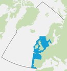
Zone Évaluée
Récapitulatif Imprimable
Contexte
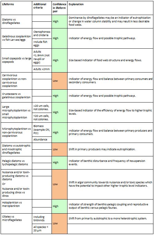
Le plancton (algues et animaux microscopiques) constitue la base des réseaux trophiques marins, il s’agit donc d’un indicateur important de l’état des écosystèmes. Les modifications des communautés planctoniques peuvent affecter des niveaux plus élevés des réseaux trophiques, tels que les mollusques et crustacés, le poisson et les oiseaux de mer, puisque ces organismes dépendent directement ou indirectement du plancton. On peut utiliser des indicateurs se fondant sur des formes de vie du plancton (c’est-à-dire des organismes possédant les mêmes traits fonctionnels; Figure 1) pour révéler les réactions des communautés planctoniques à des facteurs tels que la charge de nutriments d’origine anthropique et les modifications entraînées par le climat. Etudiées ensemble en paires ayant des rapports écologiques pertinents (voir les exemples de la Figure 1), les modifications de l’abondance relative de deux formes de vie (à savoir paire de formes de vie) peuvent indiquer des modifications des aspects fondamentaux de la fonction des écosystèmes, il s’agit notamment des liens entre les communautés pélagiques et benthiques, des flux et voies d’énergie et des interactions avec les réseaux trophiques.
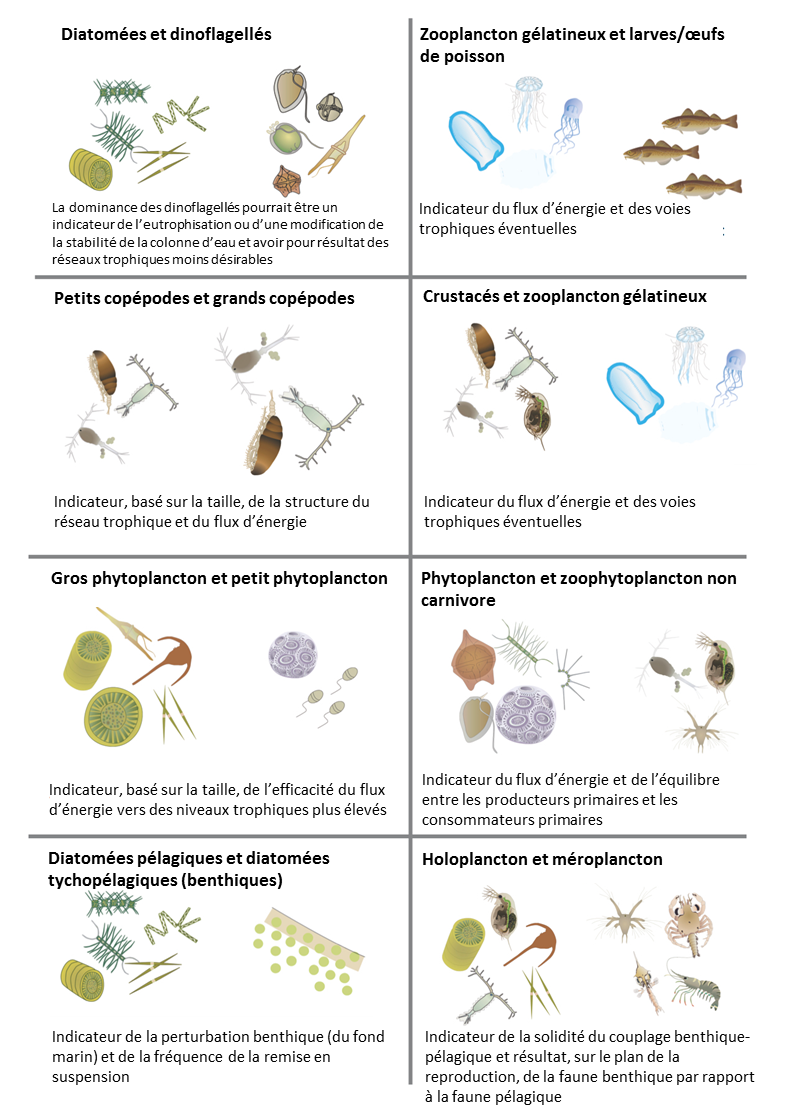
Figure 1: Paires de formes de vie planctonique et raisons écologiques de leur sélection
Des modifications de la forme de vie du phytoplancton (plancton végétal), par exemple, peuvent entraîner des modifications de la forme de vie du zooplancton (plancton animal) qui s’en nourrit. Les modifications des communautés planctoniques, au niveau régional de l’Atlantique du Nord-Est, sont étroitement liées aux conditions climatiques prédominantes. Les habitats pélagiques, qui sont définis à partir des caractéristiques clés de la colonne d’eau, sont importants pour la structure et les dynamiques des communautés planctoniques (Figure 2).
Il n’existe aucune valeur d’évaluation car il s’agit de l’évaluation d’un nouvel indicateur dans son premier stade de développement. On utilise à sa place, pour les années de 2004 à 2008 une comparaison par rapport à la période de 6 ans (2009 à 2014) pour étudier les modifications des paires de formes de vie.
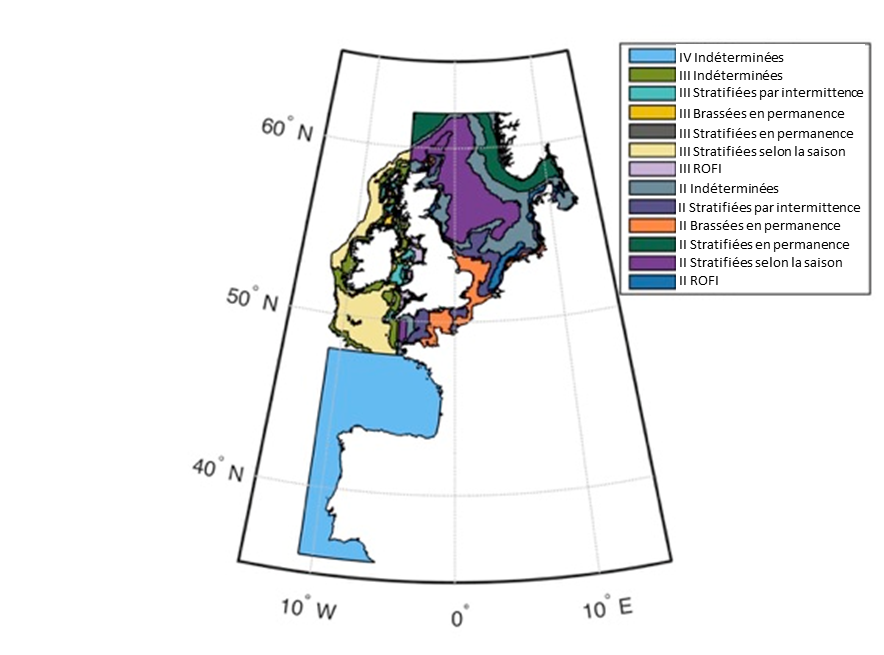
Figure 2: Zones écohydrodynamiques (EHD) dans la mer du Nord au sens large, les mers Celtiques, et le golfe de Gascogne et la côte ibérique
Les EHD sont constituées sur la base des éléments clés de la colonne d’eau, importants pour la structure et les dynamiques des communautés planctoniques. Il existe six types prédominants d’EHD basés sur la structure de la colonne d’eau: brassées en permanence toute l’année; stratifiées en permanence toute l’année; régions d’influence de l‘eau douce (ROFI); stratifiées selon la saison (pendant 6 mois environ, notamment en été); stratifiées par intermittence, et régions indéterminées (alternant de manière incohérente entre les niveaux de stratification ci-avant). Des travaux visant à définir les zones écohydrodynamiques du golfe de Gascogne et de la côte ibérique se poursuivent.
Indicators based on plankton lifeforms can be used in some hydrographic conditions to assess community response to sewage pollution (Charvet et al., 1998; Tett et al., 2008), anoxia (Rakocinski, 2012), fishing (Bremner et al., 2004), eutrophication (HELCOM, 2012) and climate change (Beaugrand, 2005). Changes in ecologically-relevant pairs of plankton lifeforms, examined together, can provide information on ecosystem structure and energy flow. The precise combinations of lifeforms comprising each lifeform pair will depend on the habitat and the objective of the indicator, for example as a measure for pelagic habitats, food webs, sea floor integrity or eutrophication. An important advantage of these plankton indicators is that the proposed concepts are relatively easily transferable to other European regional seas (Gowen et al., 2011; Rombouts et al., 2013). In practice, the use of functional groups, such as lifeforms, is often favoured over indicator species since indices of species abundance are frequently subject to large interannual variation, often due to natural physical dynamics rather than anthropogenic stressors (de Jonge, 2007). Cryptic speciation (species that look the same under a microscope) within the plankton community, alongside the limitations of identifying plankton using routine light microscopy techniques, make the true diversity of plankton communities difficult to assess at a species or genus level. Functional group abundance is often less variable because variability in the abundances of the group’s constituent species averages out. Moreover, indicators based on functional groups have been proved relevant for the description of the community’s structure and biodiversity, and are more easily inter-compared than other indicators based on taxonomy (Estrada et al., 2004; Mouillot et al., 2006; Gallego et al., 2012; Garmendia et al., 2012). When examined in ecologically-relevant pairs, lifeforms can provide an indication of changes in various aspects of ecosystem function: the transfer of energy from primary to secondary producers (changes in phytoplankton and zooplankton); the pathway of energy flow and top predators (changes in gelatinous zooplankton and fish larvae); benthic / pelagic coupling, i.e. changes in holoplankton (fully planktonic) and meroplankton (only part of the lifecycle is planktonic, the remainder is benthic) (Figure 1) (Gowen et al., 2011). Both abundance and biomass data can be used to inform lifeform pairs, depending on the lifeform in question and data availability from monitoring programmes. As the knowledge base grows, new pairs can be developed as indicators for pressures other than those currently measured. The Plankton Index (PI) of lifeform pairs has been developed to track changes in the state of the plankton in marine waters over time. The main features of the method are: (i) the grouping of species of planktonic organisms into functional types or lifeforms; (ii) the display of changes in the abundance of each of these lifeforms using a state-space approach; (iii) calculating a PI to quantify possible changes in the state of the plankton relative to baseline or starting conditions; (iv) relating trends in the PI to trends in human pressure and climate change indices. See Gowen et al. (2011) and Tett et al. (2008) for further technical information on the method. |
State-Space theory:
Tett et al. (2008) proposed to track changes in the state of the phytoplankton community by means of plots in a state-space and calculating a Plankton Community Index, referred to here as a Plankton Index (PI). The conceptual framework is that ecosystems can be viewed as systems with an instantaneous state defined by values of a set of system state variables which are attributes of the system that change with time in response to each other and external conditions. Building on this approach and plotting plankton lifeform abundance in a multi-dimensional state-space provides a means of monitoring changes in the structure of plankton communities. A state can be defined as a single point in state-space, with co-ordinates provided by the values of the set of state variables, in this case two lifeform abundances, which together are used as a pair. In the example illustrated in Figure a for diatoms and dinoflagellates, the axes of the two dimensional space are the abundance values of the two lifeforms. Each point represents the state of the ecosystem in terms of the two lifeforms at the time the water sample was collected. Subsequent samples yield additional pairs of abundance values that can be mapped onto the lifeform state-space. |
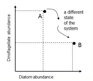
Figure a: Mapping the abundance of two lifeforms in state-space
Point A is the ecosystem state at the instant a water sample was taken and is characterised by the abundance values of two lifeforms. Another sample, taken in the same location, yields abundance values that map to a different point in the diatom-dinoflagellate state-space (point B).
The path between the two states is called a trajectory, and the condition of the phytoplankton is defined by the trajectory drawn in the state-space by a set of points. Such trajectories reflect: (i) cyclic and medium-term variability (the higher order consistencies in the plankton that result from seasonal cycles, species succession and interannual variability); and (ii) long-term variability that might result from environmental pressure. The seasonal nature of plankton production and the succession of species in seasonally stratifying seas, result in this trajectory tending in a certain direction (as plankton growth increases in the spring and declines during autumn), such that the trajectory tends towards its starting point. Given roughly constant external pressures, the data collected from a particular location over a period of years form a cloud of points in state-space that can be referred to as a regime. Long-term variability may show a persistent trend of movement away from a starting point in state-space. To define a regime, an envelope can be drawn about this group of points using a convex hull method. Because of theoretical arguments that the envelope should be doughnut-shaped with a central hole, bounding curves can be fitted outside and inside the cloud of points (Figure b). |
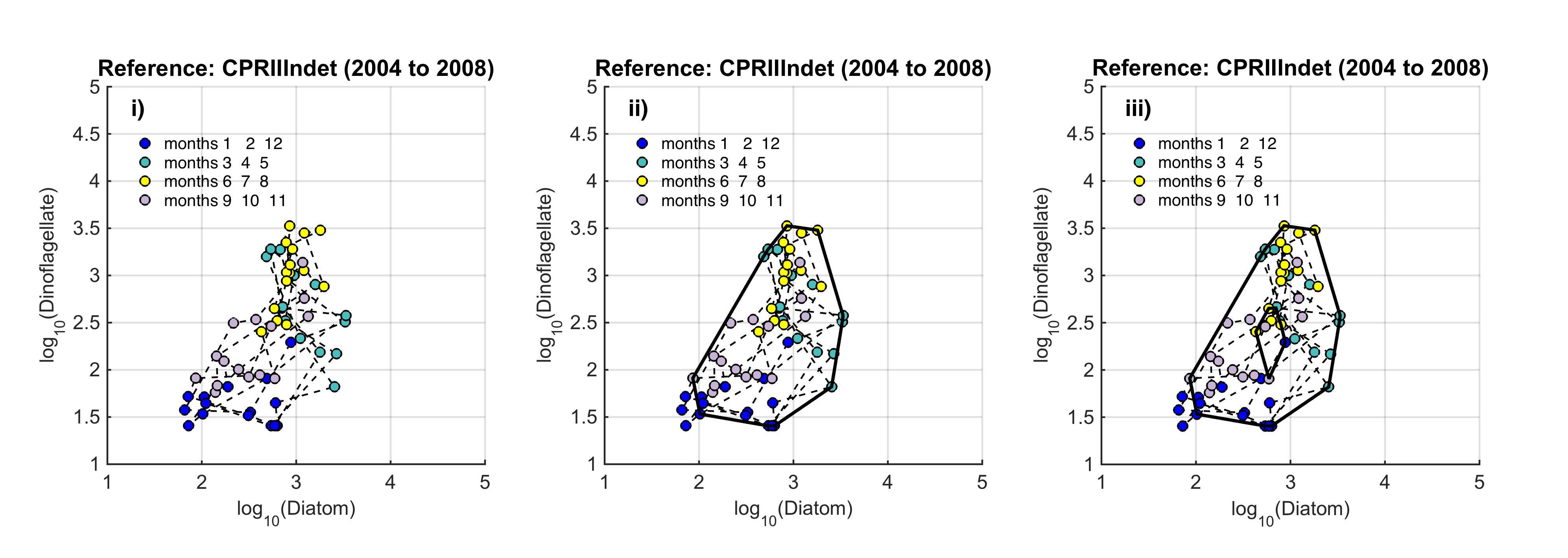
Figure b. Creating the envelope in three steps, from left (i) to right (iii): An example of a regime defined by the envelope drawn by the convex hull method
The plot is displayed on a logarithmic scale because this is a common method for showing the full extent of seasonal variability. The data are from the ecohydrodynamic zone that best represents the indeterminate area within the Greater North Sea (EHD II Indeterminate, see Figure 2). The colour of each point corresponds to the season within which it was sampled; blue = winter, aqua = spring, yellow = summer, purple = autumn.
The size and shape of the envelope are sensitive to sampling frequency and the total number of samples. Envelopes are made larger by including extreme outer or inner points, and the larger the envelope, the less sensitive it will be to change in the distribution of points in state-space and therefore to detect a change in condition. Conversely, if too many points are excluded the envelope will be small and even minor changes will result in a statistically significant difference. It is therefore desirable to exclude a proportion (p) of points, to eliminate these extremes, and so the 90-percentile was used. Envelopes are therefore drawn around the cloud of points to include a proportion (p=0.9) of the points: with the 5% of points that were most distant from the cloud's centre and the 5% of points that were closest to the centre, excluded. For a Plankton Index to be calculated, it is necessary to establish starting conditions as the basis for making comparisons. In the example shown in Figure b, data collected from the indeterminate area within the Greater North Sea (Figure 2) between 2004 and 2008, were used to create an envelope. The envelope, thus drawn (Figure c left) defines a domain in state-space that contains a set of trajectories of the diatom-dinoflagellate component of the marine pelagic ecosystem and thus represents the prevailing regime during the starting period. The next step is to map a new set of data into the starting condition state-space and compare these new data, at least a dozen points (Figure c right). The value of the PI is the proportion of new points that fall inside the envelope (or to be precise, between the inner and outer envelopes). In the example shown in Figure c, 24% or 17 of the 71 new points lie outside, and the PI is 0.76. A value of 1.0 would indicate no change, and a value of zero would show complete change, with all new points plotting outside the starting condition envelope. The envelope was made by excluding 10% of points, so some new points are expected to fall outside: 7.1 (10% of 71), in the case of the example. The exact probability of getting 17 by chance alone when only 7.1 are expected, can be calculated using a binomial series expansion, or by a chi-square calculation (with 1 df and a 1-tail test). The conclusion is that the value of 0.76, is significantly less than the expected value of 0.9, and so the condition of the phytoplankton in this region, as determined by diatoms and dinoflagellates, was statistically significantly (p<0.01) different between the two periods. |
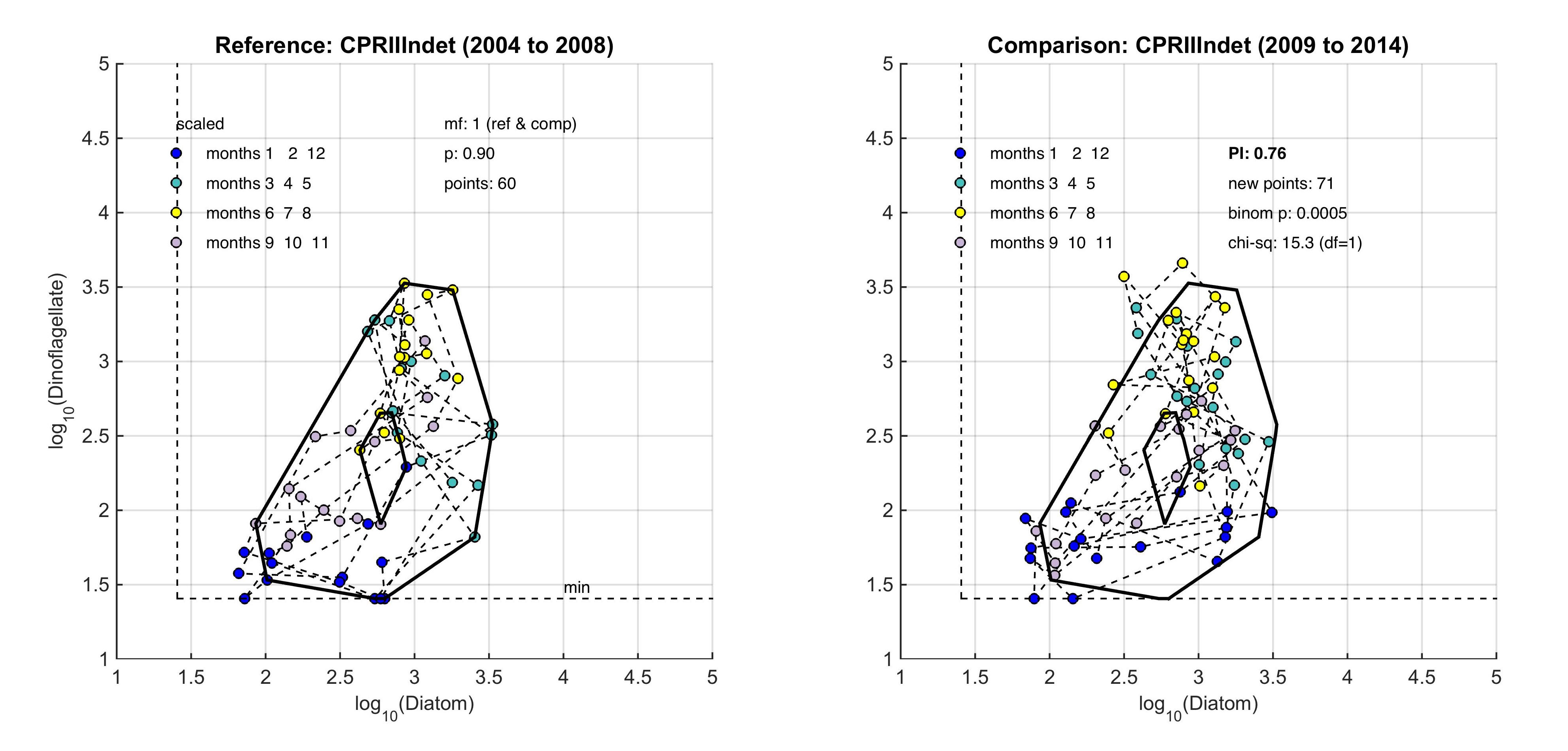
Figure c: An example for the comparison between two periods within the indeterminate area of the Greater North Sea (Figure 2), left) is the reference period of 2004–2008, right) is the comparison period of 2009–2014
The PI value of 0.76 shows a significant change between the two communities with a binomial p-value of 0.0005 (where significance = p-value <0.01).
The time series of the index is produced by comparing the starting condition envelope with data collected from each subsequent year. Two lifeforms will not be sufficient to describe all of the important characteristics of the plankton. In principle, there is no constraint to adding more lifeforms to the state-space plots (see Tett et al., 2013). The rule is that each additional lifeform must be different to those already used and the axis for each new lifeform must be drawn at right angles to all existing axes. The state-space map must therefore be drawn in as many dimensions as there are state variables (lifeforms) but this becomes complicated when considering the number of lifeforms that may need to be used to fully represent the community structure of the plankton.
|
Starting Conditions and Analysis:
The period 2004–2008 was selected to represent the starting conditions because each dataset used here (see section ‘The plankton data’) has sufficient data for that period to construct a reliable starting condition envelope. Additional European datasets will be added in the future as resources become available. This envelope represents starting conditions and not reference conditions. The starting condition envelope was compared with data from the subsequent six-year period (2009–2014). The 2009–2014 period was chosen because it is the most recent period with data and is the same temporal length as the European Union Marine Strategy Framework Directive (MSFD) assessment period.
|
Spatial Scale:
Because plankton community composition, distribution, and dynamics are closely linked to their environment, the analysis was performed at the scale of the ‘ecohydrodynamic’ zones (EHD) (van Leeuwen et al., 2015). EHDs were determined through analysis of a 50-year hindcast using the General Estuarine Transport Model (GETM) physical model of North Sea hydrodynamics (the model is at lower resolution in the Celtic Seas and is not developed for the Bay of Biscay and Iberian Coast). EHDs are constructed using density stratification, the most important large-scale physical feature in shallow shelf seas (van Leeuwen et al., 2015). Density stratification occurs when the buoyancy of surface waters (influenced by freshwater input or solar heating) is stronger than turbulence and vertical mixing, which limits vertical exchange across the pycnocline (van Leeuwen et al., 2015). The predominant EHD zone types, based on water column structure, are: permanently mixed throughout the year; permanently stratified throughout the year; regions of freshwater influence (ROFIs); seasonally stratified (for about half the year, including summer); intermittently stratified; and indeterminate regions (inconsistently alternate between the above). At the time of calculating this assessment (2016), the EHD model was more reliable and detailed for the Greater North Sea than for the Celtic Seas. The model had not been developed for the Bay of Biscay and Iberian Coast so that sub-region was considered as a single region of indeterminate status.
|
The Plankton Data:
The assessment has been carried out using phytoplankton and zooplankton data from three sources. The data submitted by the Swedish Meteorological and Hydrological Institute (SMHI) and Plymouth Marine Laboratory (PML, United Kingdom) are fixed-point time series. Four nearshore stations from SMHI were used in the analysis, which fall into the EHD zone that describes the indeterminate regions of the Greater North Sea. Both zooplankton and phytoplankton are sampled once or twice per month all year around. The PML station (L4) is 13 km offshore from Plymouth and is sampled for zooplankton and phytoplankton and a suite of other variables on a weekly basis. Unlike the fixed-point stations, data from the Continuous Plankton Recorder (CPR) survey is collected at a much broader spatial scale through ships-of-opportunity. CPR data are collected offshore and in the open ocean and are best analysed at a monthly time scale. It should be noted that all other data for this assessment come from CPR data collection on major shipping lanes. The CPR survey is coordinated by the Sir Alister Hardy Foundation for Ocean Science (SAHFOS) in the United Kingdom. Data from the different providers were not combined for analysis due to differences in sampling, plankton analysis and enumeration methods. Instead, the datasets were analysed separately. Each dataset has internal QA/QC procedures to ensure consistency and accuracy of the data. As the SMHI stations are located in the indeterminate EHD of the Greater North Sea their data were averaged for analysis. All CPR samples were averaged for each EHD type in each OSPAR sub-region. In the future, more datasets from other OSPAR Contracting Parties will be incorporated into the analysis. |
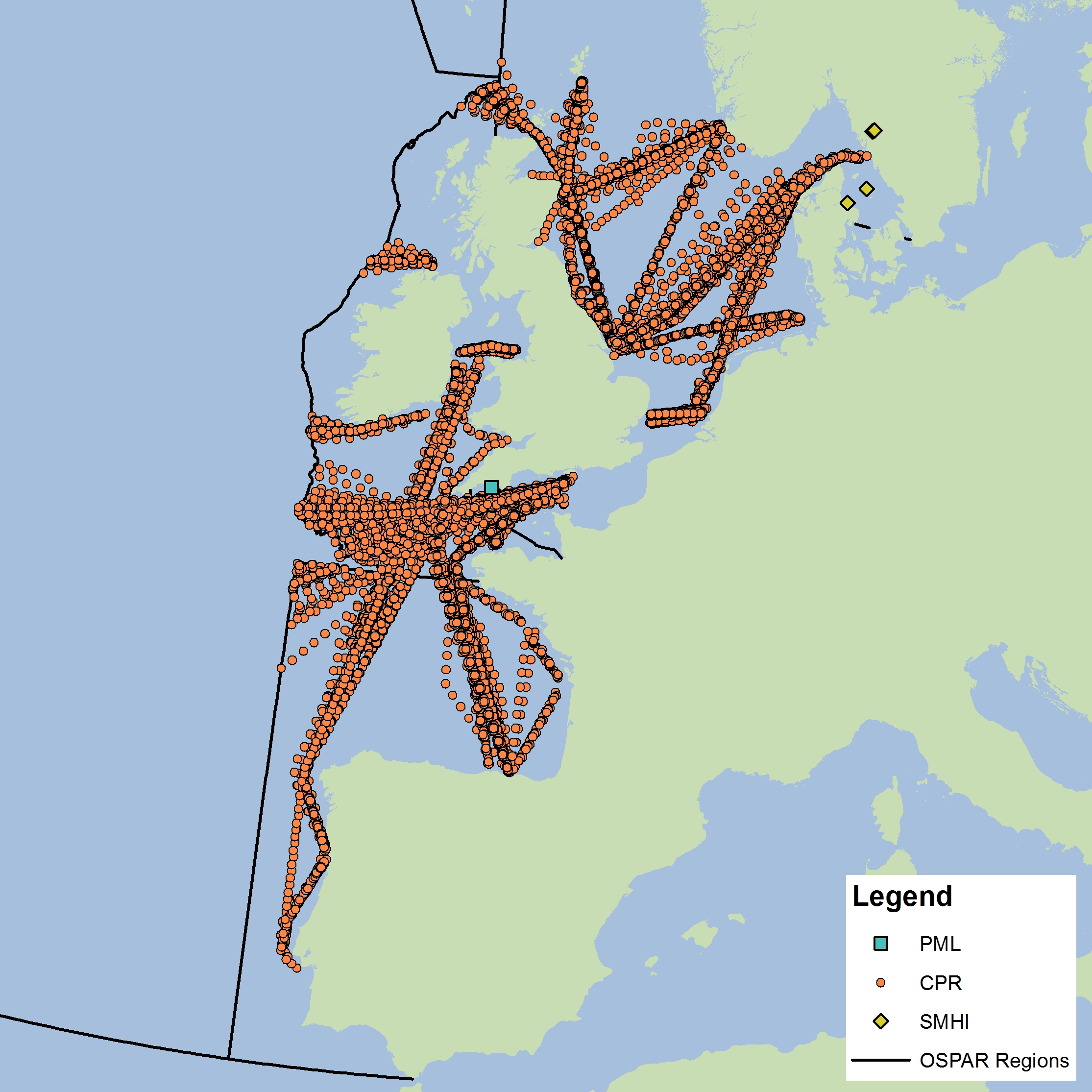
Figure d: Sample locations
The data used for this assessment were obtained from the United Kingdom (CPR and PML L4) and Sweden (SMHI). Future work will expand the plankton database to include data from additional countries.
Lifeform construction:
Each lifeform pair comprises two ecologically-relevant lifeforms, which contain common functional traits (Table a). The rationale for selecting the lifeform pairs and additional criteria containing supplementary information on lifeforms is listed in Table a. The database master species list was built by assigning functional traits to each species for a dataset and then adding additional new datasets to expand the master species list (Figure e). The species list for each new dataset was assigned a unique Aphia ID via the World Register of Marine Species (WoRMS). The new dataset’s species list was then compared with the plankton database’s master species list via Aphia IDs and any new species were identified. This process ensures that each species is only entered in the database once. The new species were then manually assigned functional traits by searching the literature; fields were left blank where functional traits for species were unknown. Once traits were assigned, the new species were added to the master species list. Queries were constructed to build lifeforms from the functional trait information (Table b). A simple method of confidence assessment was used to determine the confidence in each lifeform (Table c). Using expert opinion, each lifeform was evaluated on two characteristics: the ability to identify and speciate organisms in that lifeform using light microscopy and the understanding of the accuracy of determining traits assigned to the lifeform. For example, low confidence is assigned to the lifeform pair ‘diatoms vs autotrophic and mixotrophic dinoflagellates’ because the mixotrophic and autotrophic mode of nutrition of many dinoflagellates species is currently uncertain. Thus the accuracy of assigning the lifeform category is low. Likewise, the lifeform pair ‘carnivorous zooplankton vs non-carnivorous zooplankton’ has a low confidence designation since the feeding habits of many abundant and common zooplankton species remain unknown. Further investigation must also be conducted to decide whether both nuisance and toxin-producing lifeform pairs are required. Only pairs with two high-confidence lifeforms were used in the OSPAR reporting.
|
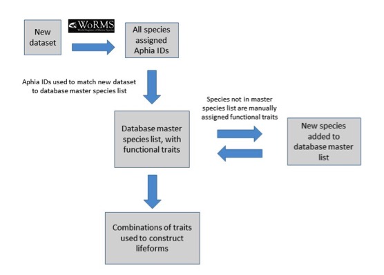
Figure e: Schematic illustrating the process undertaken to assign functional traits to species, then species to lifeforms
Each species must first be assigned a unique Aphia ID to determine whether it is already present in the master species list.
Table a: Lifeform pairs comprise two ecologically-relevant lifeforms
The ‘Additional criteria’ column contains supplementary information regarding particular lifeforms. A simple confidence rating for each lifeform pair, as described in the text, is also included.
| Lifeform | Traits | Criteria |
|---|---|---|
| Diatoms | 'Diatom' only | PhytoplanktonType=Diatom |
| Dinoflagellates | 'Dinoflagellate' only | PhytoplanktonType=Dinoflagellate |
| Gelatinous zooplankton | 'Gelatinous' only | PlanktonType=Zooplankton AND Gelatinous=Y |
| Fish larvae/eggs | 'Fish' only | ZooType=Fish |
| Carnivorous zooplankton | 'Carnivore' only | PlanktonType=Zooplankton AND Diet=Carnivore |
| Non-carnivorous zooplankton | 'Zooplankton' AND either 'Herbivore', 'Omnivore', OR 'Ambiguous' | PlanktonType=Zooplankton AND (Diet=Herbivore OR Omnivore OR Ambiguous) |
| Crustaceans | 'Crustacean' only | Crustacean=Y |
| Large phytoplankton | 'Phytoplankton' AND 'Lg' | PlanktonType=Phytoplankton AND PhytoplanktonSize=Lg |
| Small phytoplankton | 'Phytoplankton' AND 'Sm' | PlanktonType=Phytoplankton AND PhytoplanktonSize=Sm |
| Phytoplankton | 'Phytoplankton' only | PlanktonType=Phytoplankton |
| Autotrophic and mixotrophic dinoflagellates | 'Dinoflagellate' AND either 'Auto' OR 'Auto/Mixo' | PhytoplanktonType=Dinoflagellate AND (FeedingMech=Auto OR Auto/Mixo) |
| Pelagic diatoms | 'Diatom' AND 'Pelagic' | PhytoplanktonType=Diatom AND DiatomDepth=Pelagic |
| Tychopelagic diatoms | 'Diatom' AND 'Tychopelagic' | PhytoplanktonType=Diatom AND DiatomDepth=Tychopelagic |
| Nuisance and toxin-producing diatoms | 'Diatom' AND either 'Toxic' OR 'Nuisance' | PhytoplanktonType=Diatom AND (HAB = Toxic) |
| Nuisance and toxin-producing dinoflagellates | 'Dinoflagellate' AND either 'Toxic' OR 'Nuisance' | PhytoplanktonType=Dinoflagellate AND (HAB = Toxic) |
| Holoplankton | 'Holoplankton' only | Habitat=Holoplankton |
| Meroplankton | 'Meroplankton' only | Habitat=Meroplankton |
| Large copepods | 'Copepod' AND 'Lg' | Copepod=Y AND ZooSize=Lg |
| Small copepods | 'Copepod' AND 'Sm' | Copepod=Y AND ZooSize=Sm |
| Ciliates | 'Ciliate' only | PhytoplanktonType=Ciliate |
| Microflagellates | 'Dinoflagellate' AND 'Sm' | PhytoplanktonType=Dinoflagellate AND PhytoplanktonSize=Sm |
| Easy to ID/speciate | Difficult to ID/speciate | |
|---|---|---|
| Known traits | High | Low |
| Unknown traits | Low | Low |
Résultats
Cette évaluation révèle des modifications des communautés planctoniques de l’Atlantique du Nord-Est entre les périodes de 2004 à 2008 et de 2009 à 2014. Les paires de formes de vie présentent des modifications significatives dans certaines zones de l’Atlantique du Nord-Est (Figure 3) mais ceci ne signifie pas nécessairement une détérioration des conditions écologiques.
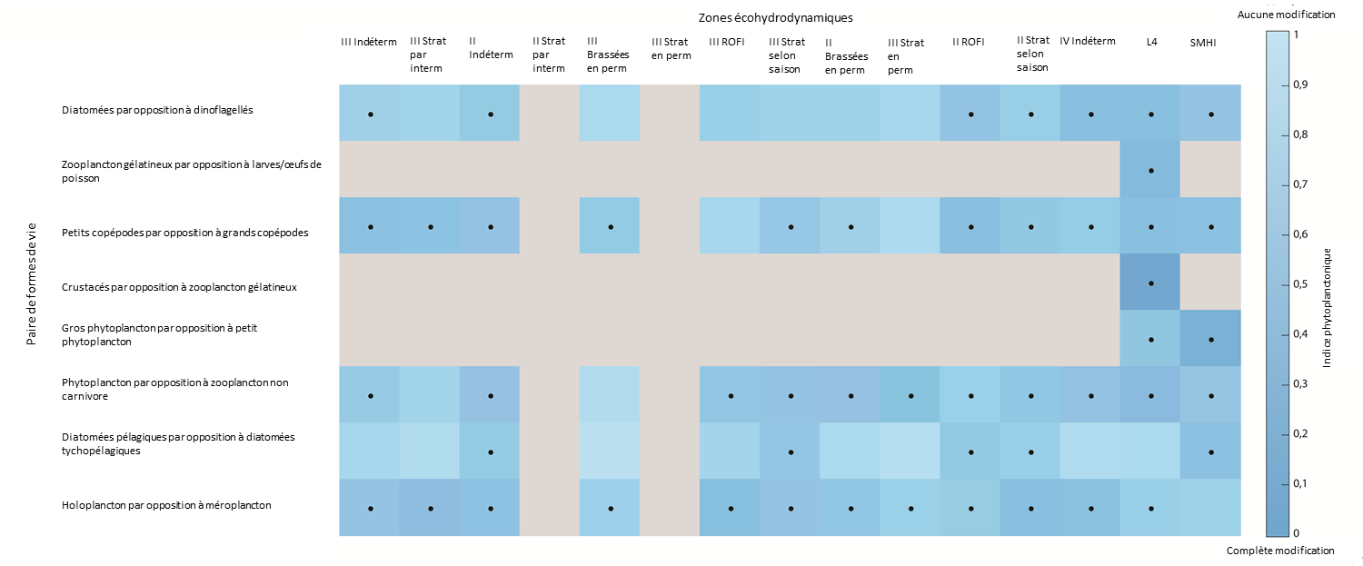
Figure 3: Modifications de l’indice planctonique entre les périodes de 2004 à 2008 et de 2009 à 2014 pour chaque paire de formes de vie
Le bleu foncé indique une modification plus prononcée. Le gris indique que les données permettant de déterminer l’indice planctonique sont insuffisantes/pas bien représentées. Les cases à pois indiquent des modifications significatives (p<0,01) depuis la période de 2004 à 2008. Les modifications de l’indice planctonique n’indiquent pas nécessairement une détérioration des conditions écologiques. Elles indiquent cependant une modification par rapport aux conditions d’origine. L’abscisse représente les zones écohydrodynamiques décrites dans la figure 2.
La paire de formes de vie « holoplancton et méroplancton » a subi des modifications significatives dans la plupart des zones, ce qui suggère des modifications des liens entre les éléments benthiques et pélagiques des écosystèmes. Des modifications se sont également produites dans la paire de formes de vie « petit copépode et grand copépode » dans de nombreuses zones, ce qui pourrait indiquer des altérations possibles de la structure du réseau trophique et des flux d’énergie. La paire de formes de vie « diatomée pélagique et diatomée tychopélagique (benthique) » n’a subi des modifications significatives que dans quelques zones, ce qui pourrait indiquer qu’il n’y a eu aucune modification importante de la remise en suspension dans la majeure partie de l’Atlantique du Nord-Est.
Il n’est pas possible actuellement d’établir des liens entre les modifications des paires de formes de vie et toute pression anthropique particulière ou autres évaluations d’indicateurs de la biodiversité.
On considère que les méthodes et les données utilisées pour cet indicateur inspirent une confiance modérée.
Figure 3 shows significant change in many lifeform pairs in many ecohydrodynamic (EHDs) zones between the starting conditions (2004–2008) and the 2009–2014 period. Even though the changes observed are statistically significant, this does not suggest that the changes are symptomatic of a deteriorating environment. It is widely acknowledged that prevailing conditions are the key driver of plankton communities in the North-East Atlantic, particularly at the relatively large EHD scale (see van Leeuwen et al., 2015, 2016). Progress towards further understanding and interpretation of the results was made during the European Union co-financed EcApRHA project coordinated by OSPAR to address gaps in biodiversity indicator development. All extended results can be downloaded here. Confidence Assessment |
Conclusion
Cette évaluation indique que les communautés planctoniques présentent une certaine variabilité pour toutes les formes de vie, ce qui est conforme à la documentation scientifique publiée sur les dynamiques du plancton.
L’évaluation de l’indicateur révèle des modifications mais des travaux supplémentaires sont nécessaires afin de tirer des conclusions sur l’ampleur, la direction et les pressions fondamentales ou les facteurs environnementaux entraînant des modifications des paires de formes de vie. Il faudra encore interpréter les résultats et affiner plus avant la méthodologie. Une vaste base de recherche revue par des pairs suggère cependant que les conditions océanographiques et climatiques prédominantes sont les forces motrices d’ensemble des modifications du plancton dans l’Atlantique du Nord-Est.
This assessment indicates spatial and temporal variability in the plankton community for all lifeforms. This is in accordance with expert knowledge on plankton dynamics from the scientific literature (McQuatters-Gollop et al., 2015). The plankton lifeform indicator has been published in the peer-reviewed literature (Tett et al., 2008) and has been developed at the sub-regional scale using data from the pan-European Continuous Plankton Recorder survey which has documented quality assurance procedures and has supported over 1000 scientific publications (McQuatters-Gollop et al., 2015). The data and methods used here are therefore considered robust and of high confidence. |
Lacunes des connaissances
Des recherches scientifiques supplémentaires sont nécessaires pour étudier l’ampleur et la direction des modifications de l’indice planctonique du point de vue de chaque paire de formes de vie, ainsi que des conséquences écologiques de telles modifications, pour chaque paire de formes de vie de chaque zone écohydrodynamique. Il y a également lieu d’envisager des liens entre la modification des paires de formes de vie et les pressions anthropiques et climatiques. Si l’on peut séparer les modifications dues aux conditions prédominantes (telles que la variabilité naturelle et le changement climatique) de celles dues aux pressions anthropiques dans chaque région, on pourra informer la prise de décisions de gestion en permettant l’application de mesures de gestion ciblées au niveau régional, si nécessaire uniquement.
The following work needs to be taken forward to address the knowledge gaps and improve the assessment provided by this indicator:
|
- Establishment of monitoring for pico and nanoplakton to provide data on a relatively data-sparse component of the plankton community.
Beaugrand, G., (2005). Monitoring pelagic ecosystems using plankton indicators. ICES Journal of Marine Science, 62: 333-338. Bremner, J., Frid, C.L.J. and Rogers, S.I., (2004). Biological traits of the North Sea benthos – Does fishing affect benthic ecosystem function? . In: P. Barnes, Thomas, J. (Editor), Benthic habitats and the effects of fishing. American Fisheries Society, Bethesda, MD, pp. 477-489. Charvet, S., Roger, M.C., Faessel, B. and Lafont, M., (1998). Biomonitoring of freshwater ecosystems by the use of biological traits. Annals of Limnology – International Journal of Limnology, 34: 455-464. de Jonge, V.N., (2007). Toward the application of ecological concepts in EU coastal water management. Marine Pollution Bulletin, 55: 407-414. Estrada, M., Henriksen, P., Gasol, J.M., Casamayor, E.O. and Pedrós-Alió, C., (2004). Diversity of Planktonic Photoautotrophic Microorganisms Along a Salinity Gradient as Depicted by Microscopy, Flow Cytometry, Pigment Analysis and DNA-based Methods. FEMS Microbiology Ecology, 49: 281-293. Gallego, I., Davidson, T.A., Jeppesen, E., Perez-Martinez, C., Sanchez-Castillo, P., Juan, M., Fuentes-Rodriguez, F., Leon, D., Penalver, P., Toja, J. and Casas, J.J., (2012). Taxonomic or ecological approaches? Searching for phytoplankton surrogates in the determination of richness and assemblage composition in ponds. Ecological Indicators, 18: 575-585. Garmendia, M., Borja, Á., Franco, J. and Revilla, M., (2012). Phytoplankton composition indicators for the assessment of eutrophication in marine waters: Present state and challenges within the European directives. Marine Pollution Bulletin, 66: 7-16. Gowen, R.J., McQuatters-Gollop, A., Tett, P., Best, M., Bresnan, E., Castellani, C., Cook, K., Forster, R., Scherer, C. and Mckinney, A., (2011). The Development of UK Pelagic (Plankton) Indicators and Targets for the MSFD. Advice to Defra, Belfast, UK, 41 pp. HELCOM, (2012). Development of the HELCOM core-set indicators Part B, GES 8/2012/7b. HELCOM, Brussels, McQuatters-Gollop, A., Edwards, M., Helaouët, P., Johns, D.G., Owens, N.J.P., Raitsos, D.E., Schroeder, D., Skinner, J. and Stern, R.F., (2015). The Continuous Plankton Recorder survey: how can long-term phytoplankton datasets deliver Good Environmental Status? . Estuarine, Coastal and Shelf Science, 162: 88-97. Mouillot, D., Spatharis, S., Reizopoulou, S., Laugier, T., Sabetta, L., Basset, A. and Chi, T.D., (2006). Alternatives to taxonomic-based approaches to assess changes in transitional water communities. Aquatic Conservation-Marine and Freshwater Ecosystems, 16: 469-482. Rakocinski, C.F., (2012). Evaluating macrobenthic process indicators in relation to organic enrichment and hypoxia. Ecological Indicators, 13: 1-12. Rombouts, I., Beaugrand, G., Fizzala, X., Gaill, F., Greenstreet, S.P.R., Lamare, S., Le Loc’h, F., McQuatters-Gollop, A., Mialet, B., Niquil, N., Percelay, J., Renaud, F., Rossberg, A.G. and Féral, J.P., (2013). Food web indicators under the Marine Strategy Framework Directive: from complexity to simplicity? Ecological Indicators, 29: 246–254. Tett, P., Carreira, C., Mills, D.K., van Leeuwen, S., Foden, J., Bresnan, E. and Gowen, R.J., (2008). Use of a phytoplankton community index to assess the health of coastal waters. ICES Journal of Marine Science, 65: 1475-1482. Tett, P., Gowen, R., Painting, S., Elliott, M., Forster, R., Mills, D., Bresnan, E., Capuzzo, E., Fernandes, T. and Foden, J. (2013) Framework for understanding marine ecosystem health. Marine Ecology Progress Series, 494, 1-27. https://doi.org/10.3354/meps10539 van Leeuwen, S., Tett, P., Mills, D. and Molen, J.v.d., (2015). Stratified and nonstratified areas in the North Sea: Long-term variability and biological and policy implications. Journal of Geophysical Research Oceans, 120: 4670-4686. |
van Leeuwen, S.M., Le Quesne, W.F. and Parker, E.R., (2016). Potential future fisheries yields in shelf waters: a model study of the effects of climate change and ocean acidification. Biogeosciences, 13: 441-454.