

Changes in Phytoplankton Biomass and Zooplankton Abundance
Background
Drifting microscopic algae and animals form the base of the pelagic food web and are a direct or indirect food source for fish, shellfish and seabirds. Planktonic organisms are highly sensitive to the physical and chemical environmental parameters, including nutrient concentrations, salinity, and temperature. These parameters are dependent on natural climatic and hydrographic variation, as well as on human-induced processes. Due to their short lifecycles, plankton respond more rapidly than higher trophic level organisms to environmental changes. Indicators based on plankton can help identify changes in plankton quantity and community structure which can therefore impact marine ecosystem structure and functioning.
The Pelagic Habitat indicator 2 (PH2) addresses “changes in phytoplankton biomass and zooplankton abundance”. This indicator provides a means of identifying changes (anomalies) in the quantities of two fundamental groups within a plankton community, phytoplankton and zooplankton (assessed by the abundance of copepods, as they are the most numerous zooplankton group). Such changes represent deviations from the assumed natural variability in a plankton time-series. Changes in phytoplankton biomass and zooplankton abundance are measured between a past comparison period (prior 2015) and a temporary assessment period (2015 – 2019). The direction of change is statistically identified as either increasing, not changing, or decreasing. This indicator has been assessed at a regional scale, using COMP4 assessment units (Enserink et al., 2019) to divide the data provided for Greater North Sea, Celtic Sea and Bay of Biscay and Iberian Coast (OSPAR Regions II, III and IV). Assimilating the results of this indicator with changes in plankton lifeforms and plankton diversity will help provide a more holistic understanding of changes occurring across pelagic habitats.
The quantity of marine plankton is, to a large extent, determined by nutrient concentrations, climate, hydrodynamic drivers and food availability (e.g., Beaugrand et al., 2009). Total phytoplankton (as biomass using chlorophyll-a or Phytoplankton Colour Index as a proxy) and zooplankton (as abundance - using total copepods abundance) represent key components of the plankton community. They account for the largest part of the plankton biomass and thus play an important role in overall plankton production, as well as grazing, lysis (auto- and viral), advection and sedimentation processes. Being at the base of the food web, plankton represent (directly or indirectly) a food resource for numerous species at higher trophic levels, such as fish of commercial interest (mackerel, herring, cod). Variability in phytoplankton biomass and zooplankton abundance can have significant impacts on the structure and function of the marine food web, as well as on ecosystem processes such as nutrient recycling. The intrinsic characteristics of plankton organisms, such as their small size, lack of commercial exploitation, short lifecycles, and a global distribution, make them essential components of monitoring programmes aiming to assess the state of marine ecosystems. Their short lifecycles and sensitivity to abiotic factors mean that plankton indicators can provide early warnings of change in the marine ecosystem (Batt et al., 2013), from both natural and human-induced change, over a wide range of temporal and spatial scales. Increased pressure on marine systems is expected to lead to greater and more frequent changes at the base of the food web. Early warnings of ecosystem change can help to prompt management actions when changes are still manageable (see Burthe et al., 2016).
Robust statistical techniques exist to identify significant components of variation and changes at multiple temporal and spatial scales for plankton. These changes may indicate major changes in the marine system involving consequences for other ecosystem components and processes. Significant changes in this indicator are evaluated through time-series analysis. One advantage of the methodology is its ease of application to any data set that can be considered ‘long enough’ to represent the temporal variability of plankton. However, since plankton dynamics are not well understood, it is difficult to decide the minimum appropriate length of a time-series for an assessment. As a starting point, it is recommended that the minimum length of a time-series should be five years, but preferably a minimum of ten years. It is also necessary that monitoring data are acquired at regular intervals through consistent sampling and analytical procedures.
The methodology for this indicator can be applied to fixed monitoring station time-series (the most common coastal monitoring in European countries) and to large-scale spatio-temporal data sets such as the Continuous Plankton Recorder (CPR) or more recently satellite data. The three data types are complementary and may provide information on different temporal / spatial scales and pressures in the future. For instance, coastal data from fixed monitoring stations can be used to identify plankton indicators that could be linked to human pressures, while large-scale spatio-temporal data in the open ocean can be used to identify plankton indicators that could be linked to large-scale hydro-meteorological changes or to indirect human pressures (e.g., fishing). An important advantage of these plankton indicators is that the concepts are relatively easily transferable to other regions (Gowen et al., 2011; Rombouts et al., 2013). For the future development of these indicators the definition of comparison periods will require knowledge of environmental and human pressure data.
The OSPAR Quality Status Report 2010 highlighted the potential impacts of climate change and other human pressures on plankton communities. Phytoplankton chlorophyll-a and phytoplankton indicator species are also assessed under the Common Procedure for the Identification of the Eutrophication Status of the OSPAR Maritime Area (OSPAR Agreement 2022-07) but there was no comparable regional assessment of phytoplankton biomass and zooplankton abundance due to the use of different assessment units divisions.
A current challenge is to separate expected natural variability from the variability induced by human pressures, a particularly difficult objective that is not yet resolved by plankton science. In the future, further development of this indicator will focus on making the link with human pressures and environmental / climate variability (see Buttay et al., 2015).
The full method employed for this indicator is further elaborated in an OSPAR guidance document for both phytoplankton and zooplankton (Aubert et al., 2017, Duflos et al., 2018, OSPAR PH2 CEMP guidelines, OSPAR Agreement 2019-06).
The methodology has been adapted since the Intermediate Assessment (IA) 2017 (mainly in the first steps of data preparation) due to the type of data used. First, phytoplankton and zooplankton are considered separately. Second, three main data types related to different acquisition systems are considered: time-series of plankton samples collected at fixed (mainly coastal) stations, plankton data from semi-autonomous collecting devices that regularly cover large spatial domains, such as the Continuous Plankton Recorder (CPR) data set, and satellite chlorophyll-a (ocean colour product) that provide a monthly synoptic view of the OSPAR Regions.
Pre-analysis steps: Specificities related to data type
Phytoplankton data
Instead of querying a particular species or group, the bulk phytoplankton community is examined through the total phytoplankton biomass. Phytoplankton biomass can be measured as biovolume, carbon content, or can be assessed through a proxy by measuring the concentration of chlorophyll-a, a pigment which is present in all phytoplankton organisms. It is also possible to derive a semi-quantitative measurement of phytoplankton biomass by analysing the Phytoplankton Colour Index (PCI), a metric of pigmentation specific to CPR data. This method estimates the green colour of the plankton community sampled onto a silk net (McQuatters-Gollop et al., 2015). Despite their shorter time-series (since 1997 with SeaWiFS derived data), satellite data were preferable for this analysis over PCI as they provide a more integrated and synoptic view with more regular monitoring and fine-scale spatial and temporal resolution which facilitated comparisons across all areas, including those not monitored by CPR. In-situ chlorophyll-a and satellite chlorophyll-a are used in this assessment as they represent the two types of data most regularly distributed in all areas (including reference stations and ocean colour data from remote sensing algorithms). For data from discrete stations no spatial aggregation was required prior to time series analysis. For non-station data (e.g., satellite, CPR), see the below section “Non-station Data”.
Zooplankton data
For zooplankton, only total copepod abundance was included in the indicator calculation. Expression of total zooplankton abundance as total copepod abundance was justified, given that copepods are readily identifiable in samples and represent the balance between production/import and mortality/export between phytoplankton and zooplankton (Budria et al., 2017). In addition, copepods are generally the most abundant and ubiquitous zooplankton taxa, both in space and time (e.g. Rombouts et al., 2009, Turner, 2004, Ikeda, 1985). In practice, the use of groups, such as copepods, is often favoured over single species as indicators (De Jonge, 2007). Indeed, some species, such as those belonging to meroplankton, can exhibit very patchy distribution and highly variable fluctuation in abundance between years. These fluctuations are often due to natural physical dynamics rather than human pressures (De Jonge, 2007). An indicator based on only one species is also unlikely to represent the whole trophic level of zooplankton communities, and which is required here for the present indicator assessment. Using a taxonomic group as broad as copepods we represent a variety of trophic interactions, characteristic of the zooplankton community, which will enable us to detect changes in the pelagic habitat. For data from discrete stations no spatial aggregation was required prior to time series analysis. For non-station data (e.g., satellite and CPR), see the “Non-station Data” section.
Non-station data
Large spatio-temporal pelagic data sets originated from satellite for phytoplankton biomass and from the CPR for zooplankton abundance. The satellite data provided by Plymouth Marine Laboratory (PML) originated from the European Space Agency Ocean Colour Climate Change Initiative using the OC5CI Chla algorithm. The OC5CI chlorophyll algorithm can be applied in case 1 - open ocean regions, as well as case 2 - coastal regions (Tilstone et al., 2022). The satellite provided by Royal Belgian Institute of Natural Sciences (RBINS) originated from the European Organisation for the Exploitation of Meteorological Satellites (EUMETSAT) using the CHL-Gons algorithm from Sentinel3/OLCI. This algorithm is developed for turbid and eutrophic waters. Prior to analysis all copepod species abundance per unit of time (within a sample) were summed to obtain total copepods abundance. The first common step of both plankton components was to aggregate data in space and time using a 1-degree grid for each month to better assess the study area. The procedure consisted of rounding latitude and longitude of samples to the nearest degree. If several sites within a pixel of the grid were acquired during the same month, the average value was calculated. The second step consisted in computing temporal interpolation of the pixels of the grid. For each cell of the grid, if more than 3 consecutive months or more than 4 non-consecutive months were missing in a year, the whole year was removed from the time-series. Thus, for time-series with 3 consecutive or 4 non-consecutive missing months within a year, temporal interpolation was processed. The temporal interpolation was particularly useful in supplementing the year-round satellite data for the North Sea, which are often missing during the winter months due to the short daylight duration (November to February).
For assessment at large spatial scale, chlorophyll-a estimation from satellite (both PML and RBINS) as well as zooplankton abundance from the Continuous Plankton Recorder (CPR, Marine Biological Association) are preferred over in situ data originated from monitoring fixed stations.
Methodology and concept:
This indicator is based on identification of phytoplankton biomass and zooplankton abundance anomalies within plankton time-series. Anomalies represent deviations from the assumed natural variability of a time-series. Thus, the greater the magnitude of the anomaly (in terms of absolute value, since anomalies can be positive or negative), the greater the change. An anomaly value of zero indicates no difference from the time-series mean (which must be de-seasonalised). To understand the changes presented (i.e., annual anomalies) and to be most useful for decision makers, annual anomalies are best interpreted with information provided by anomalies on monthly time-scales. An R-script for the plankton time series was first developed by Ibanez (reported in Berline et al., 2009), and then adapted for this assessment.
Previous assessment:
The previous assessment (OSPAR Intermediate Assessment; IA 2017) was based on the establishment and the categorisation of annual anomalies of plankton biomass. Anomalies were categorised to improve the presentation of results from a graphical perspective and to simplify the results for management use. The categorisation is based on percentiles using the 2,5, 25, 50, 75 and 97,5th percentiles for each time-series. Three categories were used: small change (anomalies within the 25–75th percentile range), important change (anomalies within the 2,5–25th percentile range and 75–97,5th percentile range) and extreme change (anomalies within the 0–2,5th percentile range and 97,5–100th percentile range). Anomalies within the small change category represent the scenario of least likely occurring significant shifts at the plankton community level, and thus the least likely to impact the marine ecosystem. Anomalies within the important change and extreme change categories have increasing potential to represent significant modifications in the plankton community and the marine ecosystem. The present assessment is based on the previous assessment methodology with some improvements since IA2017. Most of these improvements have already been described and applied in the French national MSFD assessment (Duflos et al., 2018).
Temporal trend analysis of biomass anomalies
Temporal resolution increased between IA2017 and the present assessment from yearly anomalies to monthly calculation. This change in methodology was necessary to better capture variations in phytoplankton biomass and zooplankton abundance beyond their natural cycles. This increase of temporal resolution could be achieved through monthly or higher sampling frequency.
When the data are in the format of monthly mean values, they can be fitted to the COMP4 assessment units (see the subsection Spatial scales of the assessment). Following these steps, the time-series analysis can be run. Both phytoplankton and zooplankton time-series analyses are run using the same R-script for both discrete-station data and non-station data, after the pre-analysis steps have been followed. The first step consists of identifying the mean seasonal cycle (which is called seasonality in this assessment) during the whole study period. Removing the seasonality is required in order to analyse the variations of each plankton compartment (i.e., phytoplankton biomass or zooplankton abundance) beyond their natural cycle. The second step consists in obtaining anomalies by subtracting this seasonality from the original time-series. The method used is the seasonal differentiation by the seasonal deviation methods. Finally, the cumulative sum of these anomalies was produced to detect regime shifts in the time-series for the assessment and comparison periods. A Spearman rank correlation test is now implemented to test the trend of the cumulative sum of the anomalies of the assessment and comparison periods. The correlation can move toward a significant (p≤0,05) increase in phytoplankton biomass/zooplankton abundance (0 to 1), no changes (=0) or decrease in phytoplankton biomass/zooplankton abundance (-1 to 0). The results of the Spearman rank correlation provided an indication of changes. A t-test against the cumulative sum of the anomalies of the comparison period and the assessment period provide information whether the trends are significantly different or not. These improvements to the methodology since IA2017 now allow us to define distinct comparison and assessment periods. For the QSR2023 assessment, the comparison period included all data prior to 2015 and the assessment period was set from 2015 to 2019, due to post-2019 data not yet being available across all plankton datasets.
Spatial scales
Because plankton community composition, distribution, and dynamics are closely linked to their environment, the analysis was performed at the scale of the ‘COMP4 assessment units’ (COMP4 v8a; Figure a, Table a). Assessment units within the Greater North Sea and Celtic Seas (OSPAR Regions II and III, respectively) were initially developed by Deltares and partner institutes as part of the EU Joint Monitoring Programme of the Eutrophication of the North Sea with Satellite data (JMP-EUNOSAT; Enserink et al., 2019) and further refined in the revision process of the eutrophication assessment by OSPAR expert groups ICG-EMO and TG-COMP. Assessment units with similar phytoplankton dynamics were derived from cluster analysis of satellite data for chlorophyll-a and primary production. Boundaries between assessment units were derived by relating clustering results to the best-matching gradients in environmental variables obtained from the three-dimensional hydrodynamic Dutch Continental Shelf model version 6 (DCSMv6 FM). The variables which best matched the divisions highlighted by clustering were depth, salinity, and stratification regime. Additional geographic areas were added such as the Channel, Irish Sea and Kattegat. These assessment units are a geographical representation of the conditions which best suit plankton distribution, dynamics, and community composition.
Because the Bay of Biscay and Iberian Coast (OSPAR Region IV) extended beyond the boundaries of the DCSMv6 FM, assessment units within this Region were developed using a different methodology, based on phytoplankton dynamics (Spain) and salinity dynamics (Portugal). To delineate assessment units for the Spanish coast, a polygon was created to extend from the coast to the exclusive economic zone (EEZ) boundary. Daily MODIS-Aqua Level-2 satellite images were used to calculate climatological mean values of chlorophyll-a for each pixel. K-means clustering was then used to group pixels with similar dynamics, resulting in six distinct groupings within the main Spanish polygon. Portugal’s three Water Framework Directive assessment units were extended to the boundaries of the Portuguese EEZ. These assessment units were further divided longitudinally to separate pelagic waters from coastal waters more subject to eutrophication from river influence by applying a salinity threshold, followed by a bathymetry threshold.
Figure a: COMP4 assessment units developed by JMP-EUNOSAT and OSPAR. Available at: https://odims.ospar.org/en/submissions/ospar_comp_au_2023_01/
Classification of the pelagic habitats
Following the European Commission (2017) outlining criteria and methodological standards on good environmental status of marine waters, the COMP4 assessment units and the fixed-point stations are associated with a habitat type within their corresponding OSPAR Region (Table a). Habitat identifications were processed following strict criteria according to surface mean salinity and mean depth. Four habitats were identified: variable salinity (corresponding to river plumes and regions of freshwater influence (ROFI)), coastal habitat (nearshore areas adjacent to ROFIs with mean salinity < 34,5), shelf habitat (corresponding to offshore areas with mean depth less than 200 m and mean salinity > 34,5) and oceanic/beyond shelf habitats (corresponding to offshore areas with mean depth greater than 200 m).
| Area code | Area name | Salinity (surface mean) | Depth (mean) | Habitat type | OSPAR region |
|---|---|---|---|---|---|
| ADPM | Adour plume | 34,4 | 87 | Variable salinity | IV |
| ELPM | Elbe plume | 30,8 | 18 | II | |
| EMPM | Ems plume | 31,4 | 19 | II | |
| GDPM | Gironde plume | 33,5 | 34 | IV | |
| HPM | Humber plume | 33,5 | 16 | II | |
| LBPM | Liverpool Bay plume | 30,6 | 15 | III | |
| LPM | Loire plume | 33,8 | 38 | IV | |
| MPM | Meuse plume | 29,3 | 16 | II | |
| RHPM | Rhine plume | 31,0 | 17 | II | |
| SCHPM1 | Scheldt plume 1 | 31,4 | 13 | II | |
| SCHPM2 | Scheldt plume 2 | 30,9 | 15 | II | |
| SHPM | Shannon plume | 34,1 | 61 | III | |
| SPM | Seine plume | 31,8 | 25 | II | |
| THPM | Thames plume | 34,4 | 22 | II | |
| CFR | Coastal FR Channel | 34,2 | 33 | Coastal | II |
| CIRL | Coastal IRL 3 | 34,0 | 65 | III | |
| CNOR1 | Coastal NOR 1 | 34,3 | 190 | II | |
| CNOR2 | Coastal NOR 2 | 34,0 | 217 | II | |
| CNOR3 | Coastal NOR 3 | 32,4 | 171 | II | |
| CUK1 | Coastal UK 1 | 34,5 | 60 | III | |
| CUKC | Coastal UK Channel | 34,8 | 37 | II | |
| CWAC | Coastal Waters AC | No information | No information | IV | |
| CWBC | Coastal Waters BC | No information | No information | IV | |
| CWCC | Coastal Waters CC | No information | No information | IV | |
| ECPM1 | East Coast (permanently mixed) 1 | 34,8 | 73 | II | |
| ECPM2 | East Coast (permanently mixed) 2 | 34,5 | 43 | II | |
| GBC | German Bight Central | 33,4 | 39 | II | |
| IRS | Irish Sea | 33,7 | 65 | III | |
| KC | Kattegat Coastal | 25,7 | 21 | II | |
| KD | Kattegat Deep | 27,6 | 50 | II | |
| NAAC1A | NorAtlantic Area NOR-NorC1 | No information | No information | IV | |
| NAAC1B | NorAtlantic Area NOR-NorC1 | No information | No information | IV | |
| NAAC1C | NorAtlantic Area NOR-NorC1 | No information | No information | IV | |
| NAAC1D | NorAtlantic Area NOR-NorC1 | No information | No information | IV | |
| NAAC2 | NorAtlantic Area NOR-NorC2 | No information | No information | IV | |
| NAAC3 | NorAtlantic Area NOR-NorC3 | No information | No information | IV | |
| OC | Outer Coastal DEDK | 33,4 | 27 | II | |
| SAAC1 | SudAtlantic Area SUD-C1 | No information | No information | IV | |
| SAAC2 | SudAtlantic Area SUD-C2 | No information | No information | IV | |
| SAAP2 | SudAtlantic Area SUD-P2 | No information | No information | IV | |
| SNS | Southern North Sea | 34,3 | 32 | II | |
| ASS | Atlantic Seasonally Stratified | 35,2 | 134 | Shelf | III, IV |
| CCTI | Channel Coastal shelf tidal influenced | 34,8 | 40 | II | |
| CWM | Channel well mixed | 35,1 | 77 | II, III | |
| CWMTI | Channel well mixed tidal influenced | 35,0 | 59 | II | |
| DB | Dogger Bank | 35,1 | 28 | II | |
| ENS | Eastern North Sea | 34,8 | 43 | II | |
| GBCW | Gulf of Biscay coastal waters | 34,6 | 53 | IV | |
| GBSW | Gulf of Biscay shelf waters | 34,9 | 107 | IV | |
| IS1 | Intermittently stratified 1 | 35,3 | 138 | II, III | |
| IS2 | Intermittently stratified 2 | 35,1 | 102 | II | |
| NAAP2 | NorAtlantic Area NOR-NorP2 | No information | No information | IV | |
| NAAPF | NorAtlantic Area NOR-Plataforma | No information | No information | IV | |
| NNS | Northen North Sea | 35,0 | 121 | II | |
| NT | Norwegian Trench | 34,1 | 349 | II | |
| SAAP1 | SudAtlantic Area SUD-P1 | No information | No information | IV | |
| SK | Skagerrak | 31,8 | 134 | II | |
| SS | Scottish Sea | 35,1 | 89 | II, III | |
| ATL | Atlantic | 35,3 | 2291 | Oceanic / Beyond shelf | II, IV, V |
| NAAO1 | NorAtlantic Area NOR-NorO1 | No information | No information | IV | |
| OWAO | Ocean Waters AO | No information | No information | IV | |
| OWBO | Ocean Waters BO | No information | No information | IV | |
| OWCO | Ocean Waters CO | No information | No information | IV | |
| SAAOC | Sudatlantic Area SUD-OCEAN | No information | No information | IV | |
| Stonehaven | No information | No information | Coastal | II | |
| Loch Ewe | No information | No information | Variable salinity | III | |
| L4 | No information | No information | Coastal | II | |
| N14 Falkenberg | No information | No information | Coastal | II | |
| Anholt | No information | No information | Coastal | II | |
| Slaggö | No information | No information | Coastal | II | |
| E2CO | No information | No information | Coastal | IV | |
| E3VI | No information | No information | Coastal | IV | |
| A17 | No information | No information | Shelf | II | |
| E1GI | No information | No information | Shelf | IV | |
| E2GI | No information | No information | Shelf | IV | |
| E3GI | No information | No information | Shelf | IV | |
| E1CU | No information | No information | Shelf | IV | |
| E2CU | No information | No information | Shelf | IV | |
| E3CU | No information | No information | Shelf | IV |
Data provided and used in this assessment
Satellite data for the Greater North Sea (OSPAR Region II) and the Celtic Seas (OSPAR Region III) were provided by the Royal Belgian Institute for Natural Sciences and Plymouth Marine Laboratory. Missing values or gaps smaller than 4 months were interpolated by cubic spline method. In addition to satellite data, in situ chlorophyll-a data from stations were provided by Plymouth Marine Laboratory for L4 station (Channel well mixed assessment unit), by Marine Scotland Science for Stonehaven and Loch Ewe fixed stations, by the Swedish Meteorological and Hydrological Institute and by Aarhus University (Kattegat and Skagerrak assessment units) and by Landesamt für Landwirtschaft, Umwelt und ländliche Räume des Landes Schleswig-Holstein and the Niedersächsischer Landesbetrieb für Wasserwirtschaft, Küsten und Naturschutz (North Sea). In the Bay of Biscay and Iberian Coast (OSPAR Region IV), data were provided by the Instituto Espanol de Oceanografia from a set of fixed stations located in the Bay of Biscay and Iberian Coast.
In addition, non-station data from the CPR have been provided respectively by the Marine Biological Association. CPR data were used for calculating the PH2 indicator on zooplankton (copepod) abundance. However, the CPR Phytoplankton Colour Index (PCI) was not used in the end for phytoplankton biomass assessment, despite CPR providing the longer time series that would be possible to compare to phytoplankton time-series. For phytoplankton biomass, it is more suitable to use satellite data as they provide a monthly integrated and synoptic view of chlorophyll-a across the Greater North Sea and the Celtic Seas (OSPAR Regions II and III respectively).
In a few cases, the spatially distributed data resulted in localised groupings of samples being extrapolated across much larger assessment units (see distribution of CPR samples in Figure d (i) ( PH1 indicator assessment ), as was the case for CPR data along the west of Scotland (Intermittently Stratified 1) and Ireland (Atlantic Seasonally Stratified).
Additional data from fixed stations were provided by Belgium, the Netherlands, and the United Kingdom, however, due to some time-series being shorter than the comparison-assessment period or located outside OSPAR Regions, some data were not used in this assessment. Data from ongoing monitoring within OSPAR assessment regions will be used in the future (e.g., VLIZ data from Belgium). Table b provides a list of the data used for this assessment.
| Contracting Party | Institute | Dataset name | Date range | Sampling frequency |
|---|---|---|---|---|
| Belgium | Royal Belgium Institute of Natural Sciences (RBINS) | CHL_RBINS | 2009-2020 | Daily |
| Denmark | Aarhus University | NOVANA chlorophyl data | 2009-2020 | Fortnightly |
| Germany | Landesamt für Landwirtschaft, Umwelt und ländliche Räume des Landes Schleswig-Holstein (LLUR) | OSPAR_LLUR-SH Phytoplankton Biomass_2010-2020 | 2010-2020 | Fortnightly |
| Niedersächsischer Landesbetrieb für Wasserwirtschaft, Küsten und Naturschutz (NLWKN) | OSPAR_NLWKN_1999-2019 | 1999-2019 | Fortnightly to higher frequency | |
| Spain | Instituto Espanol de Oceanografia (IEO) | IEO_RADIALES_Chla | 1989-2020 | Monthly |
| IEO_RADIALES_Zoo | 1991-2018 | Monthly | ||
| Sweden | Swedish Meteorological and Hydrological Institute (SMHI) | National data_SMHI phytoplankton biomass | 1986-2020 | Monthly |
| National data_SMHI_ zoo | 1996-2020 | Monthly | ||
| United Kingdom | Environment Agency (EA) | EA CHL 2000-2020 | 2000-2020 | Weekly or higher frequency |
| Marine Biological Association (MBA) | CPR dataset 1960-2019 | 1960-2019 | Weekly or higher frequency | |
| Marine Scotland Science (MSS) | MSS Loch Ewe biomass | 2002-2020 | Weekly | |
| MSS Loch Ewe zooplankton | 2002-2017 | Weekly | ||
| MSS Stonehaven biomass | 1997-2020 | Weekly | ||
| MSS Stonehaven zooplankton | 1999-2020 | Weekly | ||
| Plymouth Marine Laboratory (PML) | PML_L4 chl a | 1992-2020 | None | |
| PML_L4 zooplankton | 1988-2020 | Fortnightly to higher frequency | ||
| PML ICES satellite | 1997-2016 | Monthly |
Relationship between environmental pressures and phytoplankton biomass / zooplankton abundance
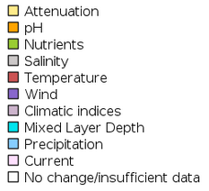
Environmental variables were selected according to their relevance and availability for plankton to determine the most important pressure in phytoplankton biomass and zooplankton abundance changes. While all the variables listed in Table c were used for modelling phytoplankton biomass, nutrients were removed from the model explaining zooplankton abundance. The set of environmental variables used originated from different models targeting the North-East Atlantic area.
The first step consisted of evaluating long-term links to pressures and to avoid excluding the first several decades of many plankton time-series due to missing values. To achieve this, the method used multiple random forest regressions to impute missing values based on collinearities among observed values in the predictors. For each variable containing missing values the algorithm generated a separate regression model based on all the other predictors. To improve imputation performance, a numeric variable representing ‘month’ was included in this step to better predict the consistent seasonal patterns in some variables. This step was performed using ‘missRanger’ R package (Mayer and Mayer 2019).
Then, values for each environmental variable were calculated as the mean of monthly mean gridded values (modelled and remotely sensed) within each COMP4 assessment unit. For fixed-point stations, mean values were calculated from all measurements within a 5-nautical mile radius of the station. Where in situ data were available (total nitrogen, nitrate, phosphate, total phosphorous, silicate) they were evaluated instead of the modelled environmental variables. For Atlantic Multidecadal Oscillation (AMO) and North Atlantic Oscillation (NAO), monthly values were applied identically across all assessment units since these variables have basin-scale influence likely to cover the entire assessment region.
Finally, a random forest algorithm was applied to evaluate which was the best combination of environmental variable for phytoplankton biomass / zooplankton abundance prediction. The algorithm is based on the combination of predictions made by multiple regression trees (here, k = 1000 trees) with the optimal tree (defined as the best combination of variables) obtained by majority voting. It is however important to note that the random forest algorithm may be affected by correlated variables.
Prior to analysis, the original datasets were split into two subsets resulting in a training set and a test set. The training set was used for the selection of the best combination while the test set was used to validate the predictions. The training set consisted of data from the comparison period (prior to 2015) while the test set consisted of data from the assessment period (from 2015 to 2019).
For map visualisation, some variables were aggregated together. Total nitrogen, nitrate, phosphate, total phosphorus, N:P ratio and silicate were pooled under the term "nutrient”. The same procedure was applied for AMO and NAO which were pooled under the term "Climate indices".
It is important to keep in mind that on the pressures presented below, pH is not an independent variable. Indeed, the pH of seawater is controlled by the concentration of dissolved inorganic carbon (DIC). Changes in pH can be linked to changes in phytoplankton activity, since phytoplankton ingest DIC to fuel growth and reproduction, but also to the concentration of atmospheric carbon dioxide, the main driver of global warming. Consequently, increases of phytoplankton biomass could increase seawater pH and vice versa. However, a change in pH can adversely affect phytoplankton biomass.
Table c: list of environmental variables used as pressures.
| Variable name | Description | Abbreviation | Source |
|---|---|---|---|
| Sea surface temperature | Temperature of surface layer, as measured by satellite | sst | International Comprehensive Ocean-Atmosphere Data Set (ICOADS): https://psl.noaa.gov/data/gridded/data.coads.1deg.html |
| Salinity | Salinity of the surface layer | sal | European Regional Seas Ecosystem Model (ERSEM; NWSHELF_MULTIYEAR_PHY_004_009; https://doi.org/10.48670/moi-00059) |
| Total Oxidised Nitrogen | Total oxidised nitrogen concentration in surface layer | totn | In situ data from Marine Scotland Science (MSS): https://doi.org/10.7489/1881-1 |
| Nitrate | Nitrate concentration of the surface layer | ntra | European Regional Seas Ecosystem Model (ERSEM; NWSHELF_MULTIYEAR_BGC_004_011): https://doi.org/10.48670/moi-00058); |
| Phosphate | Dissolved inorganic phosphate concentration of the surface layer | phos | European Regional Seas Ecosystem Model (ERSEM; NWSHELF_MULTIYEAR_BGC_004_011): https://doi.org/10.48670/moi-00058); ); In situ data from Plymouth Marine Laboratory (PML): https://www.westernchannelobservatory.org.uk/l4_nutrients.php and Marine Scotland Science (MSS): https://doi.org/10.7489/1881-1 https://www.westernchannelobservatory.org.uk/l4_nutrients.php |
| Total phosphorous | Total phosphorous concentration of the surface layer | totp | In situ data from Aarhus University (Svendsen et al. 2005) |
| N:P ratio | The ratio of molar nitrogen concentration to molar phosphorus concentration | np | Derived from: https://www.westernchannelobservatory.org.uk/l4_nutrients.php and Marine Scotland Science (MSS): https://doi.org/10.7489/1881-1 |
| Silicate | Dissolved silicate concentration of the surface layer | Si | In situ data from Marine Scotland Science (MSS): https://doi.org/10.7489/1881-1; |
| Wind speed | Wind speed (proxy of turbulence) | wspd | International Comprehensive Ocean-Atmosphere Data Set (ICOADS); https://psl.noaa.gov/data/gridded/data.coads.1deg.html |
| Mixed layer depth | Surface layer in which density is nearly homogeneous with depth | mld | European Regional Seas Ecosystem Model (ERSEM; NWSHELF_MULTIYEAR_PHY_004_009; https://doi.org/10.48670/moi-00059) |
| Light attenuation | The extinction coefficient for the visible light in the water column | attn | European Regional Seas Ecosystem Model (ERSEM; NWSHELF_MULTIYEAR_BGC_004_011): https://doi.org/10.48670/moi-00058) https://www.westernchannelobservatory.org.uk/l4_nutrients.php https://www.westernchannelobservatory.org.uk/l4_nutrients.php |
| Precipitation | Rate of precipitation | precip | International Comprehensive Ocean-Atmosphere Data Set (ICOADS); https://psl.noaa.gov/data/gridded/data.coads.1deg.html |
| Current velocity | Current velocity in the surface layer | cvel | European Regional Seas Ecosystem Model (ERSEM; NWSHELF_MULTIYEAR_PHY_004_009; https://doi.org/10.48670/moi-00059) |
| pH | Sea water pH reported on total scale | pH | European Regional Seas Ecosystem Model (ERSEM; NWSHELF_MULTIYEAR_BGC_004_011): https://doi.org/10.48670/moi-00058) https://www.westernchannelobservatory.org.uk/l4_nutrients.php https://www.westernchannelobservatory.org.uk/l4_nutrients.php |
| NAO | The North Atlantic Oscillation is a weather phenomenon over the North Atlantic Ocean of fluctuations in the difference of atmospheric pressure at sea level between the Icelandic Low and the Azores High | nao | National Oceanic and Atmospheric Administration (NOAA): https://www.ncdc.noaa.gov/teleconnections/nao/ |
| AMO | The Atlantic Multidecadal Oscillation is the theorised variability of the sea surface temperature of the North Atlantic Ocean on the timescale of several decades | amo | National Oceanic and Atmospheric Administration (NOAA); https://psl.noaa.gov/data/timeseries/AMO/ |
Integration of indicator results:
A primary objective of this indicator assessment was to integrate results to facilitate an understanding of changes occurring across pelagic habitat types within OSPAR Regions II, III and IV. This required indicator results for each of these OSPAR Regions to be integrated according to the following pelagic habitat categories: variable salinity, coastal, shelf, and oceanic / beyond shelf. This categorisation of COMP4 assessment units and fixed-point stations is described in Table a. To meet this objective, we focused on the primary direction of change detected across assessment units and fixed-point stations within each pelagic habitat category for each of the 2 plankton components highlighted in this assessment. We then reported the mean confidence, spatial representativeness, and most likely links to environmental pressures.
As an example, changes in zooplankton were assessed across 6 COMP4 areas and 4 fixed-point stations representing coastal habitats within OSPAR Region II. If 4 decreasing trends, 3 increasing trends, and 3 instances of no trend were detected across these locations, we would report a decreasing net trend and the proportion of assessment units studied where this trend was detected, in this case 0,4.
The spatial representativeness of the result corresponds the proportion of the total number of COMP4 assessment units considered in the analysis, in this case 6, out of the total number of possible COMP4 assessment units representing coastal habitats within the OSPAR Region, in this case 12. Therefore, the spatial representativeness of the result would be 0,5. Note that fixed-point station datasets do not contribute to this score.
Finally, to report links to environmental pressures which can drive changes in PH2 components for the net trend, we ranked environmental variables for each location based on their relative variable importance, with 1 assigned to the variable with highest importance, 2 to the variable with second highest importance and so on. For locations where the net trend was increasing, we calculated the mean rank of each environmental variable and reported the variable with the lowest mean rank.
Addressing PH2 quality status
In order to deliver a clear and comprehensive message to the scientific and non-scientific community, the results of the indicator were summarised by their quality status per habitat within each OSPAR region. The quality status had been defined by the change in indicator value for each plankton component according to assessment threshold and / or the impact of anthropogenic pressures and climate change on the indicator change (McQuatters-Gollop et al., 2022). Thus, the quality status resulted in 4 categories: Not good, Unknown, Good, and Not assessed. Table d gives the detailed explanation of the different categories.
Table d: Categorization of the quality status and their associated narratives
| Quality status categories | |
|---|---|
| Not good | Indicator value is below assessment threshold, or change in indicator represents a declining state, or indicator change is linked to increasing impact of anthropogenic pressures (including climate change), or indicator shows no change but state is considered unsatisfactory |
| Unknown | No assessment threshold and/or unclear if change represents declining or improving state, or indicator shows no change but uncertain if state represented is satisfactory |
| Good | Indicator value is above assessment threshold, or indicator represents improving state, or indicator shows no change but state is satisfactory |
| Not assessed | Indicator was not assessed in a region due to lack of data, lack of expert resource, or lack of policy support. |
Results
This assessment identified changes in phytoplankton biomass and zooplankton abundance at regional and local scales. Among the 64 COMP4 areas, significant changes were found in 39 assessment units for phytoplankton biomass (Figure 1) and in 22 assessment units for zooplankton abundance (Figure 2).
 and the comparison period (station data: 1992–2014; non-station data: 1997–2014). Hatched areas were characterised by significant changes (p≤0,05) in phytoplankton biomass between the comparison and the assessment periods. White areas indicate no data or insufficient data to assess the area.")
Figure 1: Trend in phytoplankton biomass anomalies between the assessment period (2015–2019) and the comparison period (station data: 1992–2014; non-station data: 1997–2014). Hatched areas were characterised by significant changes (p≤0,05) in phytoplankton biomass between the comparison and the assessment periods. White areas indicate no data or insufficient data to assess the area.
 and the comparison period (1960–2014). Hatched areas were characterised by significant changes (p≤0,05) in zooplankton abundance between the comparison and the assessment periods. White areas indicate no data or insufficient data to assess the area. Results of Intermittently Stratified 1 (Scotland) and Atlantic Seasonally Stratified (Ireland) assessment units should be interpreted cautiously as CPR samples were extrapolated across much larger assessment units.")
Figure 2: Trend in zooplankton abundance anomalies between the assessment period (2015–2019) and the comparison period (1960–2014). Hatched areas were characterised by significant changes (p≤0,05) in zooplankton abundance between the comparison and the assessment periods. White areas indicate no data or insufficient data to assess the area. Results of Intermittently Stratified 1 (Scotland) and Atlantic Seasonally Stratified (Ireland) assessment units should be interpreted cautiously as CPR samples were extrapolated across much larger assessment units.
Both phytoplankton biomass anomalies and zooplankton abundance anomalies exhibited decreasing trends across the majority of COMP4 units assessed. The assessment period (2015-2019) was marked by strong and significant decreases in phytoplankton biomass across 32 assessment units, while increases were documented in 7 areas. For zooplankton abundance, strong decreases occurred across 13 areas, whereas abundance increased in 8 areas and 1 area had no change. A large decrease in phytoplankton biomass occurred in open ocean waters (Atlantic areas and Bay of Biscay), in the English Channel and a few North Sea areas (mainly the Eastern North Sea and the Norwegian Trench) whereas biomass increased in a large part of the North Sea areas (Elbe, Ems and Humber Plumes, Northern and Southern North Sea, Dogger Bank). For zooplankton, a large decrease in abundance occurred in offshore waters such as open ocean waters (Atlantic areas and Bay of Biscay), the English Channel and a large part of the North Sea (except coastal waters and the Norwegian Trench). Significant increase of phytoplankton biomass occurred in coastal and shelf habitats of the Greater North Sea and Celtic Seas (Coastal UK channel and Coastal UK 1, Irish and Scottish Seas, East Coat permanently mixed 1, Norwegian Trench).
In agreement with the results for this indicator presented in the IA2017, phytoplankton biomass has continued to increase in the North Sea except in the Eastern part of the North Sea (Eastern North Sea, German Bight Central and Outer Coastal DEDK). Zooplankton abundance exhibited a large decrease in the stations from open ocean waters (Atlantic areas and Bay of Biscay), some regions of the English Channel (Channel well mixed and Channel well mixed tidal influenced) and North Sea waters (Northern North Sea, Dogger Bank, Eastern North Sea, German Bight Central and Outer Coastal DEDK). An increase in abundance was mainly observed along the English coasts and in the Norwegian Trench. Although IA2017 reported a negative trend in zooplankton abundance for the Southern North Sea, the current assessment period (2015–2019) detected no significant change in zooplankton abundance for this area. The results may be subject to variations from the existing literature possibly due to differences in spatial aggregation prior to analysis.
Links between phytoplankton biomass (Figure 3) / zooplankton abundance (Figure 4) and climate change linked pressures control were evidenced in the Celtic Seas and the Bay of Biscay and Iberian Coast. Increasing sea surface temperature (SST), decreasing wind speed, decrease of light attenuation and increasing mixed layer depth were linked to decrease in phytoplankton biomass and zooplankton abundance. Furthermore, decreases of phytoplankton biomass and zooplankton abundance in coastal and shelf habitats of the Celtic Seas were associated with decreasing pH. In the variable salinity, coastal and shelf habitats of the Greater North Sea, nutrients (nitrate, phosphate, N:P ratio), considered as a proxy of eutrophication, were the most important variables in the phytoplankton biomass changes. Impact of eutrophication may be significant in this region and further investigations must be carried out with OSPAR’s ICG-Eut group to better understand the underlying relationships. Regarding these relationships, quality status of most habitats within the OSPAR Regions was "Not good". Only variable salinity habitats in the Greater North Sea and the Celtic Seas had an “Unknown" quality status. Further details for this section can be found in the extended results.
Anomalies percentile in the time-series
For the previous assessment (IA2017) annual anomalies in a time-series were categorised as either small, intermediate, or important changes. This categorisation could be used as an “early warning” signal of change. Some examples of anomalies from the Dogger Bank are displayed for phytoplankton biomass (Figure b) and for zooplankton abundance (Figure c) using the previous assessment methods based on percentiles. This method focused on the amplitude of monthly deviation from mean conditions, rather than assessing a trend through time. For example, extreme values [<2,5 or >97,5] accompanied large changes in the plankton, triggering further investigation into understanding such changes.
 for the Dogger Bank area over the period 1997-2019. Three colours have been attributed to each category: Light blue (small change), blue (intermediate change) and dark blue (important change).")
Figure b: Monthly anomalies of phytoplankton biomass (non-station data from satellite) for the Dogger Bank area over the period 1997-2019. Three colours have been attributed to each category: Light blue (small change), blue (intermediate change) and dark blue (important change).
 for the Dogger Bank area over the period 1960-2019. Three colours have been attributed to each category: Light blue (small change), blue (intermediate change) and dark blue (important change).")
Figure c: Monthly anomalies of zooplankton abundance (non-station data from the CPR) for the Dogger Bank area over the period 1960-2019. Three colours have been attributed to each category: Light blue (small change), blue (intermediate change) and dark blue (important change).
Integration of phytoplankton biomass and zooplankton abundance trends
The results of the current assessment have indicated 3 patterns of change between phytoplankton and zooplankton (Figure d): (i) a simultaneous decrease in both phytoplankton biomass and zooplankton abundance, (ii) increase in phytoplankton biomass and decrease in zooplankton abundance or decrease in phytoplankton biomass and increase in zooplankton abundance, and (iii) a simultaneous increase of phytoplankton biomass and zooplankton abundance.

Figure d: Integration between PH2 phytoplankton and zooplankton trends within the different COMP4 assessment units and at the different fixed stations.
Downward arrow represents simultaneous decrease of phytoplankton biomass and zooplankton abundance (pattern i). Upward arrow represents simultaneous increase of phytoplankton biomass and zooplankton abundance (pattern iii). Bidirectional arrows represent increase of one plankton component while the second component decreases and vice versa (pattern ii).
The first pattern (i) was observed in the open ocean waters (Atlantic areas), as well as in the Channel well mixed and Channel well mixed tidal influenced areas, in the south-eastern part of the North Sea (e.g., Eastern North Sea, German Bight Central) as well as in some fixed-points (i.e. L4, Loch Ewe, E1GI, E2GI, Anholt and Slaggö).
The second pattern (ii) was recorded in the Northern North Sea, the Dogger Bank, in the Coastal Waters of Ireland, Outer Coastal waters, along the Southern English coasts (Coastal waters of Southern England), the Irish and Scottish Seas, and in the North Sea (East Coast of England, Intermittently stratified waters, Coastal waters of Norway and the Norwegian Trench). This pattern was found in only one monitoring station: Stonehaven location.
The third pattern (iii) was observed in the Elbe and Ems plumes and in the fixed points in the Skagerrak (i.e., Slaggö, A17) and the Iberian coast (i.e., E1CU, E2CU, E3CU, E3GI and E2CO).
Relation between pressures and indicator
In the Greater North Sea, modelling results have revealed nutrients (dissolved inorganic phosphate, nitrogen, and the balance between nitrogen and dissolved inorganic phosphate) as the most important pressures affecting changes in phytoplankton biomass for the three types of habitats (variable salinity, coastal and shelf). Variable salinity habitat was marked by a decrease in phosphate which in turn was high correlated with a decrease of phytoplankton biomass (see also Gohin et al., 2020). Faster reduction of phosphorous than nitrogen occurred in both coastal and shelf habitats resulting in increasing N:P ratio. In both habitats, these conditions occurred while phytoplankton biomass decreased. Zooplankton abundance was rather linked to direct or indirect climatic conditions. Despite increasing, SST were reported as the most important variable for zooplankton abundance decrease in the variable salinity habitat, the relation was insignificant thus changes did not occur during the assessment period. Finally, decreasing mixed layer depth (MLD) was linked with decreasing zooplankton abundance in coastal habitat, decreasing MLD was linked with increasing zooplankton abundance in shelf habitats.
In the Celtic Seas, the current assessment showed that decreasing pH was most likely linked with phytoplankton biomass decrease in coastal habitat and in shelf habitats for both phytoplankton biomass and zooplankton abundance (further explanations on the relationship between pH and phytoplankton biomass are given in the subsection Relationship between environmental pressures and phytoplankton biomass / zooplankton abundance). Changes in pH can be linked to changes in phytoplankton activity, since phytoplankton ingest dissolved inorganic carbon (DIC) to fuel growth and reproduction, but also to the concentration of atmospheric carbon dioxide, the main driver of global warming. However, for reasons described above, the relationship between pH and phytoplankton biomass should be evaluated cautiously and further analysis is necessary to quantify phytoplankton’s contribution to pH variability. Indicator results in variable salinity habitats also reflected a reduction in phytoplankton biomass due to decreasing nitrate concentration. The increase in zooplankton abundance in the coastal habitat was linked to natural climatic condition. Finally, decrease in zooplankton abundance in variable salinity habitats was linked to decrease of current velocity.
In the Bay of Biscay and Iberian Coast (OSPAR Region IV), changes in both phytoplankton biomass and zooplankton abundance were most strongly linked to climatic conditions. While phytoplankton biomass decreased in shelf habitats due to increasing mixed layer depth over the last decades, phytoplankton biomass also decreased in oceanic habitats, associated with a decrease in light attenuation and thus shallowing of the euphotic zone. Surprisingly, zooplankton abundance in coastal and oceanic habitats was positively correlated with SST. Results indicated that abundance increased as well as SST in coastal habitat whereas abundance and SST both decreased in oceanic habitats. Finally, decreases in zooplankton abundance in shelf habitats of the Bay of Biscay and Iberian Coast were linked to increasing mixed layer depth.
The quality status of the pelagic habitats within OSPAR Regions was addressed following the links between pressures and PH2 indicator results (Table e). Despite relationships with environmental variables remaining unclear, climate change and decrease in pH were linked with the indicators within coastal and shelf habitats of the Celtic Seas and within coastal, shelf and Oceanic / beyond shelf habitats of the Bay of Biscay and Iberian Coast. Consequently, the quality status within these habitats is “Not good”. The faster reduction in phosphorus compared to nitrogen has increased the N:P ratio which in turns impacted the PH2 indicator. This was the case for coastal and shelf habitats of OSPAR Region II. As a consequence of the imbalance between nitrogen and phosphorus, this might be related to eutrophication, and the quality status of the habitat in which this observation was made was also determined to be “Not good”. Finally, where other parameters were linked with changes in phytoplankton biomass and zooplankton abundance (e.g., variable salinity habitats of the Greater North Sea and the Celtic Seas), it was more difficult to establish the origin of the pressure. Quality status of the habitat was therefore categorised as “Uncertain”.
Table e: Integration of the indicator results for the Greater North Sea, the Celtic Seas and the Bay of Biscay and Iberian Coast. Column names are described as follows: Dir: the net direction of change in the plankton component (upward arrow: increasing trend, equality sign: no trend, downward arrow: decreasing trend), Trend: the percentage of assessment units exhibiting the respective trend (if no results were reported for assessment units, stations are used), Change: a logical variable (TRUE/FALSE) to report whether a net trend is likely given the significance of the results, Pressure: the environmental pressure with the greatest mean rank for the respective trend, Rank: the mean rank of the environmental pressure indicated under Pressure, nSt: the total number of monitoring fixed stations considered, nCOMP4: The total number of COMP4 assessment units considered, totCOMP4: The total number of potential COMP4 assessment units for the habitat category, spatialRep: the spatial representativeness score of the analysis.
OSPAR Region | Habitat | Plankton component | Dir | Trend | Change | Pressure | Rank | nSt | nCOMP4 | totCOMP4 | Spatial Rep |
The Greater North Sea | Variable salinity | Phytoplankton | ↓ | 60% | TRUE | phosp | 2.8 | 1 | 9 | 9 | 100% |
Zooplankton | ↓ | 100% | FALSE | sst | 1.0 | 1 | 0 | 9 | 0% | ||
Coastal | Phytoplankton | ↓ | 92% | TRUE | np | 4.0 | 1 | 12 | 12 | 100% | |
Zooplankton | ↑ | 40% | TRUE | mld | 2.8 | 4 | 6 | 12 | 50% | ||
Shelf | Phytoplankton | ↓ | 75% | TRUE | np | 2.3 | 1 | 11 | 11 | 100% | |
Zooplankton | ↓ | 67% | TRUE | mld | 2.7 | 0 | 7 | 11 | 64% | ||
Oceanic | Phytoplankton | NA | |||||||||
Zooplankton | NA | ||||||||||
The Celtic Seas | Variable salinity | Phytoplankton | ↓ | 100% | TRUE | ntra | 2.0 | 1 | 2 | 2 | 100% |
Zooplankton | ↓ | 100% | TRUE | cvel | 1.0 | 1 | 0 | 2 | 0% | ||
Coastal | Phytoplankton | ↓ | 67% | TRUE | pH | 1.7 | 0 | 3 | 3 | 100% | |
Zooplankton | ↑ | 67% | TRUE | AMO | 2.0 | 0 | 3 | 3 | 100% | ||
Shelf | Phytoplankton | ↓ | 100% | TRUE | pH | 3.5 | 0 | 4 | 4 | 100% | |
Zooplankton | ↓ | 75% | TRUE | pH | 2.5 | 0 | 4 | 4 | 100% | ||
Oceanic | Phytoplankton | NA | |||||||||
Zooplankton | NA | ||||||||||
The Bay of Biscay and Iberian Coast | Variable salinity | Phytoplankton | NA | ||||||||
Zooplankton | NA | ||||||||||
Coastal | Phytoplankton | ↓ | 100% | TRUE | NAO | 1.0 | 1 | 0 | 12 | 0% | |
Zooplankton | ↑ | 100% | TRUE | sst | 2.5 | 2 | 0 | 12 | 0% | ||
Shelf | Phytoplankton | ↑ | 43% | TRUE | wspd | 1.0 | 6 | 1 | 6 | 17% | |
Zooplankton | ↓ | 100% | TRUE | mld | 3.0 | 0 | 2 | 6 | 33% | ||
Oceanic | Phytoplankton | ↓ | 100% | TRUE | attn | 1.0 | 0 | 1 | 6 | 17% | |
Zooplankton | ↓ | 100% | TRUE | sst | 1.5 | 0 | 2 | 6 | 33% |
Conclusion
This assessment identifies changes in phytoplankton biomass and zooplankton abundance at regional (COMP4 assessment units) and local (discrete monitoring stations) scales. The results highlight a general decrease in phytoplankton biomass and zooplankton abundance at the regional scale. However, at the local scale, observed phytoplankton biomass has been increasing since the previous assessment in the North Sea and zooplankton abundance has also been increasing along the coasts of the United Kingdom and in the Norwegian trench. Possible links with climate change were reported especially in coastal, shelf and oceanic habitats of the Greater North Sea and the Celtic Seas. Nutrients had been linked to the indicator especially in the Greater North Sea. Future investigations are needed to explore connections with relevant Pelagic Habitat, Food Web and Eutrophication indicators.
This assessment identifies changes in phytoplankton biomass and zooplankton abundance at regional (COMP4 assessment units) and local (discrete monitoring stations) scales. The results highlight a general decrease in phytoplankton biomass and zooplankton abundance at the regional scale. However, at the local scale, observed phytoplankton biomass has been increasing since the previous assessment in the North Sea and zooplankton abundance has also been increasing along the coasts of the United Kingdom and in the Norwegian trench. Possible links with climate change were reported especially in coastal, shelf and oceanic habitats of the Greater North Sea and the Celtic Seas. Eutrophication has been linked to the indicator especially in the Greater North Sea. Future investigations are needed to explore connections with relevant Pelagic Habitat and Food Web indicators.
Knowledge Gaps
Recommendations for future work are as follows: 1. Inclusion of additional datasets, particularly for the Bay of Biscay and Iberian Coast; 2. Compare to relevant Pelagic Habitat and Food Web indicators to better address the extent of change; 3. Methodology improvement needs to be continued to define more precisely the natural cycle of phytoplankton biomass and zooplankton abundance; 4. Refine the use of satellite data and improve coherence with the eutrophication assessments; and 5. Refine the links between PH2 and pressures.
Further development of this indicator is needed, particularly on the following points:
- Inclusion of additional data sets to improve the confidence of indicator’s assessment results: especially for the Bay of Biscay and Iberian Coast. In addition, increased zooplankton monitoring is needed in variable salinity habitats. Finally, there is a need to include additional datasets to allow comparison between the different monitoring strategies.
- Comparison to relevant Pelagic Habitat and Food Web indicators to facilitate of impacts through the food web.
- Improve coherence and integration between the PH2 indicator and relevant indicators within HASEC group.
- Integration of dataset originated from different chl-a methods: continual assessment of characterising the differences in chl-a methodologies is required.
- Improve the methodology for defining the natural cycle and subsequently for the trend characterisation and spatial and temporal confidence of the results.
- Refinement of the use of remote sensing data for improving coherence with the OSPAR eutrophication assessments at different spatial and temporal scales.
- Refine the links between PH2 and pressures to identify the origin of the pressures.
Inclusion of additional data sets:
Recommendations were made in the IA2017 regarding spatial gaps in the Bay of Biscay and Iberian Coast and they are still relevant for the current assessment. In addition, in the current assessment some habitats within OSPAR Regions were lacking data. In particular, there is a need for: zooplankton data for variable salinity habitats in the Greater North Sea and the Celtic Seas and both phytoplankton and zooplankton data for variable salinity and coastal habitats in the Bay of Biscay and Iberian Coast.
In addition to ensure the perennity of existing time series, future research and monitoring studies should address the various gaps in monitoring data coverage because these will be a limiting factor for the development of the indicators. Semi-automated methods such as in vivo multi-spectral fluorometry and flow cytometry (Houliez et al., 2012; Bonato et al., 2016; Thyssen et al., 2015, Louchart et al., 2020), supplemented by automated image acquisition and analysis which allow higher spatial and temporal resolution should also be considered within existing monitoring programmes. In addition, implementation of these innovative techniques on seasonal (see Jouandet et al., 2020) or monthly sampling programs (e.g., Aardema et al., 2019) can help address pelagic community dynamics in offshore waters thus providing information to define the quality status of not assessed areas or assessed areas with low sampling confidence. Furthermore, inclusion of size fractionated chl-a could be integrated to provide a more precise view of phytoplankton biomass. Size fractionated chl-a could also be useful to integrate Pelagic Habitats indicators (this indicator and the indicator ‘ Changes in plankton lifeforms ’) since a recommendation to investigate picoplankton and nanoplankton emerged in the previous version of PH1/FW5 indicator.
Comparison to relevant Pelagic Habitat and Food Web Eutrophication indicators:
Further work is also needed to integrate pelagic habitat indicators (this indicator, and the indicators on ‘ Changes in Phytoplankton and Zooplankton Communities ’ and ‘ Changes in Plankton Diversity ’) since this will provide greater confidence in the assessment of changes in plankton, and in their integration with indicators of other ecosystem components, in particular food web indicators. PH2 is a bulk indicator, with the highest level of integration among the Pelagic Habitat indicators (McQuatters-Gollop et al., 2017). Whilst PH2 represents the link between the stocks and the fluxes within the pelagic food webs, it does not account for variability in photosynthetic rates and the actual flow of carbon through the system. Further research on the use of primary production (FW2), as a direct indicator of carbon flow through the food web, should be explored.
Improve coherence and integration with relevant eutrophication indicators:
Being at the bottom of the trophic network, plankton is highly sensitive to their changing environment. In this context, there is a need to improve the linkage with relevant eutrophication indicators from OSPAR’s Hazardous Substances and Eutrophication Committee (HASEC) such as the nutrient inputs indicator . Future investigations will help to address the importance of nutrient inputs within the sub-division of the different OSPAR Regions. Furthermore, it is important to establish better coherence between the PH2 indicator and the chlorophyll-a concentration indicator across multiple criteria: data collection (similar data should be used to maintain consistency in results), spatial resolution (similar spatial resolution should be maintained across related indicators), and temporal resolution (consistency should be maintained across related indicators in terms of whether they examine year-round time-series, or productive months only).
Integration of dataset originated from different chl-a methods:
As far as future research is concerned, continual assessment of characterising the differences in Chl-a methodologies is required (e.g., between fluorometric, spectrophotometric, HPLC and in situ fluorometers [which are prone to quenching] plus CPR colour scale index).
Methodology improvement:
The current assessment is built on the assumption that phytoplankton biomass and zooplankton abundance fluctuate over a consistent annual cycle. However, plankton have large year-to-year variability, and this pattern of variability differs across ecosystems and habitats. For example, periodicities of 12 or 6 months or less have been reported. Shifts in the typical annual cycle have also been detected in the past. Future development should therefore focus on investigating the annual cycle for non-stationary datasets (e.g., Winder and Cloern, 2010) and applying this information to de-trend time-series data. Furthermore, it is crucial to investigate the potential change of seasonality over time. Once the annual mean cycle has been removed, the trend analysis can be conducted using linear modelling. Although this methodology is widely accepted, this does not always match with the dataset. Trends can be linear, cubic, quadratic or absent. Consequently, it is necessary to propose an evaluation tool to define more accurately the type of relationship of the de-trended data over time.
Refinement of the use of remote sensing data:
For future assessments, it would be beneficial to examine satellite data at a finer spatial scale, and improve methods for using satellite remote sensing data in turbid and eutrophic water bodies. This will be particularly useful in variable salinity and coastal habitats of the Greater North Sea, which are typically characterised by high turbidity. It is also important to maintain coherence across multiple criteria: data collection (similar data should be used to maintain consistency in results), spatial resolution (similar spatial resolution should be maintained across related indicators, such as PH1/FW5, PH3, FW2 and chlorophyll-a concentration indicator ), and temporal resolution (consistency should be maintained across related indicators in terms of whether they examine year-round time-series, or productive months only). It is also important to maintain similar consistency about whether to use temporal interpolation to fill gaps for unsampled months which often occur during winter.
Refine the pressure-PH2 relationship:
The origins of the different pressures are unclear at this stage. Despite evidence from literature, future work should make the distinction between natural versus human induced pressure as well as the origin of natural pressures (e.g., nutrient originating from river run-off or benthic origin or Atlantic flow).
In addition, introduction of a lag into the variable selection is needed to test for delayed effects of environmental pressures on phytoplankton biomass and zooplankton abundance (e.g., the effects of winter nutrient concentrations on phytoplankton biomass during the growing season).
Aardema, H. M., Rijkeboer, M., Lefebvre, A., Veen, A., & Kromkamp, J. C. (2019). High-resolution underway measurements of phytoplankton photosynthesis and abundance as an innovative addition to water quality monitoring programs. Ocean Science, 15(5), 1267-1285.
Aubert A., Rombouts I., Artigas F., Budria A., Ostle C., Padegimas B., McQuatters-Gollop A. 2017, “Combining methods and data for a more holistic assessment of the plankton community”, as a contribution to the EU Co-financed EcApRHA project (Applying an ecosystem approach to (sub) regional habitat assessments), deliverable No. 1.2.
Batt, R.D., Brock, W.A., Carpenter, S.R., Cole J.J., Pace M.L., Seekell D.A., 2013. Asymmetric response of early warning indicators of phytoplankton transition to and from cycles. Theor Ecol., 6: 285. Available at: https://doi.org/10.1007/s12080-013-0190-8
Beaugrand G, Luczak C, Edwards M (2009) Rapid biogeographical plankton shifts in the North Atlantic Ocean. Glob Change Biol 15:17901790ift
Berline L., Ibanez F., Grosjean P. 2009. Roadmap for zooplankton time series analysis. SESAME WP1 report. 20p.
Bonato, S., Christaki, U., Lefebvre, A., Lizon, F., Thyssen, M., and Artigas, L. F. (2015). High spatial variability of phytoplankton assessed by flow cytometry, in a dynamic productive coastal area, in spring: The eastern English Channel. Estuarine, Coastal and Shelf Science, 154, 214-223.
Budria, A., Aubert, A., Rombouts, I., Oslte, C., Atkinson, A., Widdicombe, C., Goberville, E., Artigas., L.F., Johns, D., Padegimas, B., Corcoran, E., McQuatters-Gollop, A. (2017). Cross-linking plankton indicators to better define GES of pelagic habitats. EcApRHA Delivrable WP1.4. 54 pp.
Burthe, S. J., Henrys, P. A., Mackay, E. B., Spears, B. M., Campbell, R., Carvalho, L., Dudley, B., Gunn, I. D. M., Johns, D. G., Maberly, S. C., May, L., Newell, M. A., Wanless, S., Winfield, I. J., Thackeray, S. J. and Daunt, F. 2016. Do early warning indicators consistently predict nonlinear change in long-term ecological data?. J Appl Ecol, 53: 666–676. Available at: https://doi.org/10.1111/1365-2664.12519
Buttay L., Miranda A., Casas G., González-Quirós R., Nogueira E. 2015. Long-term and seasonal zooplankton dynamics in the northwest Iberian shelf and its relationship with meteo-climatic and hydrographic variability. Journal of Plankton Research 38(1), 106-121
De Jonge V.N. 2007. Toward the application of ecological concepts in EU coastal water management. Marine Pollution Bulletin 55, 407-414.
Duflos M., Wacquet G., Aubert A., Rombouts I., Mialet B., Devreker D., Lefebvre A., Artigas L.F. 2018. Évaluation de l’état écologique des habitats pélagiques en France métropolitaine. Rapport scientifique pour l’évaluation 2018 au titre du descripteur 1 de la DCSMM. 333 pp.
Enserink, L., Blauw, A., van der Zande, D., Markager S. (2019). Summary report of the EU project ‘Joint monitoring programme of the eutrophication of the North Sea with satellite data’ (Ref: DG ENV/MSFD Second Cycle/2016). 21 pp.
European Commission, 2017. Commission decision (EU) 2017/848 of 17 May 2017 laying down criteria and methodological standards on good environmental status of marine waters and specifications and standardised methods for monitoring and assessment, and repealing Decision 2010/477/EU. Official Journal of the European Union L, 125: 43–74.
Gohin, F., Bryère, P., Lefebvre, A., Sauriau, P. G., Savoye, N., Vantrepotte, V., Bozec, Y., Cariou, T., Conan, P., Coudray, S., Courtay, G., Françoise, S., Goffart, A., Hernández Fariñas, T., Lemoine, M., Piraud, A., Raimbault, P., & Rétho, M. (2020). Satellite and in situ monitoring of Chl-a, Turbidity, and Total Suspended Matter in coastal waters: experience of the year 2017 along the French Coasts. Journal of Marine Science and Engineering, 8(9), 665.
Gowen R.J., McQuatters-Gollop A., Tett P.M., Bresnan E., Castellani C., Cook K., Forster R., Scherer C., Mckinney A. 2011. The Development of UK Pelagic (Plankton) Indicators and Targets for the MSFD, Belfast, 2011.
Houliez, E., Lizon, F., Thyssen, M., Artigas, L. F., & Schmitt, F. G. (2012). Spectral fluorometric characterization of Haptophyte dynamics using the FluoroProbe: an application in the eastern English Channel for monitoring Phaeocystis globosa. Journal of Plankton Research, 34(2), 136-151.
Ikeda, T. (1985). Metabolic rates of epipelagic marine zooplankton as a function of body mass and temperature. Marine Biology, 85(1), 1-11.
Jouandet, M. P., Lebourg, E., Bruaut, M., Dédécker, C., Louchart, A., Gómez, F., Nowaczyck, A., Wacquet, G., Lizon, F., Crouvoisier, M., Cornille, V., Lefebvre, K., Bouchaud, F., Lécuyer, E., Mériaux, X., Cauvin, A., Didry, M., Delabre, J., Duflos, M., and Artigas, L. F. (2020). Résultats des campagnes océanographiques 2017-2019 en Mers Celtiques et Manche Mer du Nord: Test pour la mise en place du Programme de Surveillance DCSMM. 113 pp.
Louchart, A., deBlok, R., Debuschere, E., Gomez, F., Lefebvre, A., Lizon, F., Mortelmans, J., Rijkeboer, M., Schmitt, F.G., Deneudt, K., Veen, A., and Artigas, L.F. (2020). Automated techniques to follow the spatial distribution of Phaeocystis globosa and diatoms spring blooms in the Channel and North Sea, Proceedings of the ICHA2018 (18th International Conference on Harmful algae, Nantes 21-26 October 2018), 4 pp.
Mayer, M., & Mayer, M. M. (2019). Package ‘missRanger’. R Package.
McQuatters-Gollop, A., Edwards, M., Helaouët, P., Johns, D.G., Owens, N.J.P., Raitsos, D.E., Schroeder, D., Skinner, J., and Stern, R.F., 2015. The Continuous Plankton Recorder survey: how can long-term phytoplankton datasets deliver Good Environmental Status? Estuarine, Coastal and Shelf Science, 162:88-97
McQuatters-Gollop, A., Johns, D. G., Bresnan, E., Skinner, J., Rombouts, I., Stern, R., .Aubert, A., Johansen, M., Bedford, J., and Knights, A., (2017). From microscope to management: the critical value of plankton taxonomy to marine policy and biodiversity conservation. Marine Policy, 83, 1-10.
McQuatters-Gollop, A., Guérin, L., Arroyo, N.L., Aubert, A., Artigas, L.F., Bedford, J., Corcoran, E., Dierschke, V., Elliott, S.A.M., Geelhoed, S.C.V., Gilles, A., Gonzalez-Irusta, J.M., Haelters, J., Johansen, M., Le Loc’h, F., Lynam, C.P., Niquil, N., Meakins, B., Mitchell, I., Padegimas, B., Pesch, R., Preciado, I., Rombouts, I., Safi, G., Schmitt, P., Schückel, U., Serrano, A., Stebbing, P., De la Torriente, A., Vina-Herbon, C. (2022). Assessing the state of marine biodiversity in the Northeast Atlantic. Ecological Indicators, 141, 109148.
OSPAR. 2017. Changes in Phytoplankton Biomass and Zooplankton Abundance. Available at: https://oap.ospar.org/en/ospar-assessments/intermediate-assessment-2017/biodiversity-status/habitats/plankton-biomass/
OSPAR (in prep). OSPAR Agreement 2019-06. Coordinated Environmental Monitoring and Assessment Programme Guidelines for assessing changes in phytoplankton biomass and zooplankton abundance. Available at: www.ospar.org
Rombouts I., Beaugrand G., Fizzala X., Gaill F., Greenstreet S.P.R., Lamare S., Le Loc’h F., McQuatters-Gollop A., Mialet B., Niquil N., Percelay J., Renaud F., Rossberg A.G. and Féral J.P., 2013. Food web indicators under the Marine Strategy Framework Directive: from complexity to simplicity? Ecological Indicators, 29: 246–254.
Rombouts, I., Beaugrand, G., Ibaňez, F., Gasparini, S., Chiba, S., & Legendre, L. 2009. Global latitudinal variations in marine copepod diversity and environmental factors. Proceedings of the Royal Society B: Biological Sciences, 276(1670), 3053-3062.
Svendsen, L., L. van der Bijl, S. Boutrup, and B. Norup. 2005. NOVANA. National Monitoring and Assessment Programme for the Aquatic and Terrestrial. and number: NERI Technical Report.
Thyssen, M., Alvain, S., Lefebvre, A., Dessailly, D., Rijkeboer, M., Guiselin, N., Creach, V., and Artigas, L. F. (2015). High-resolution analysis of a North Sea phytoplankton community structure based on in situ flow cytometry observations and potential implication for remote sensing. Biogeosciences, 12(13), 4051-4066.
Tilstone, G. H., Land, P. E., Pardo, S., Kerimoglu, O., & Van der Zande, D. (2022). Threshold indicators of primary production in the north-east Atlantic for assessing environmental disturbances using 21 years of satellite ocean colour. Science of The Total Environment, 158757.
Turner, J.T. (2004). The importance of small planktonic copepods and their roles in pelagic marine food webs. Zoological studies 43: 255-266
Winder, M., and Cloern, J. E. (2010). The annual cycles of phytoplankton biomass. Philosophical Transactions of the Royal Society B: Biological Sciences, 365(1555), 3215-3226.
Contributors
Lead Authors: Arnaud Louchart, Matthew Holland, Abigail McQuatters-Gollop and Luis Felipe Artigas
Supported by: OSPAR Pelagic Habitat Expert group, Intersessional Correspondence Group on the Coordination of Biodiversity Assessment and Monitoring, Biodiversity Committee and the OSPAR Secretariat.
Delivered by
This work was co-funded by the European Maritime and Fisheries Fund through the project: “North-east Atlantic project on biodiversity and eutrophication assessment integration and creation of effective measures (NEA PANACEA)”, financed by the European Union’s DG ENV/MSFD 2020, under agreement No. 110661/2020/839628/SUB/ENV.C.2.
 |  |
Citation
Louchart, A., Holland, M., McQuatters-Gollop, A. and Artigas, L. F. 2023. Changes in Phytoplankton Biomass and Zooplankton Abundance. In: OSPAR, 2023: The 2023 Quality Status Report for the Northeast Atlantic. OSPAR Commission, London. Available at: https://oap.ospar.org/en/ospar-assessments/quality-status-reports/qsr-2023/indicator-assessments/changes-plankton-biomass-abundance
| Assessment type | Indicator Assessment |
|---|---|
| Summary Results | https://odims.ospar.org/en/submissions/ospar_plankton_mass_abun_msfd_2022_06/ |
| SDG Indicator | 14.2 By 2020, sustainably manage and protect marine and coastal ecosystems to avoid significant adverse impacts, including by strengthening their resilience, and take action for their restoration in order to achieve healthy and productive oceans |
| Thematic Activity | Biological Diversity and Ecosystems |
| Relevant OSPAR Documentation | OSPAR Agreement 2010-03 The North-East Atlantic Environment Strategy. Strategy of the OSPAR Commission for the Protection of the Marine Environment of the North-East Atlantic 2010–2020 |
| Date of publication | 2023-06-30 |
| Conditions applying to access and use | https://oap.ospar.org/en/data-policy/ |
| Data Snapshot | https://odims.ospar.org/en/submissions/ospar_plankton_changes_snapshot_2022_06/ |
| Data Results | https://odims.ospar.org/en/submissions/ospar_plankton_changes_results_2022_06/ |