

Extent of Physical Disturbance to Benthic Habitats: Fisheries with mobile bottom-contacting gears
Background
Benthic habitats comprise marine organisms living within or on sediments, rock or biogenic reefs and undertaking essential ecological processes and functions to support healthy ecosystems. In addition, benthic habitats are key components of marine food webs, supporting populations of commercially important fish and shellfish species, and providing a major food source for predators. The diversity of seafloor habitats is influenced by factors such as depth, light penetration, substrate type and currents on the seabed. Such variables and conditions contribute to a high habitat heterogeneity, with biological communities having varying levels of sensitivity to physical pressures. Some habitats are very sensitive (e.g., fragile coral gardens), whereas others are more resistant (able to withstand disturbance or stress without changing character); and resilient (able to recover from disturbance or stress) to physical pressure (e.g., mobile sands) (Tyler-Walters et al., 2018). Previous analyses have shown widespread disturbance in benthic habitats (OSPAR, 2017a, McQuatters-Gollop, et al., 2022). Seafloor physical disturbance, caused by pressures associated with human activities, such as bottom-contact fishing, aggregate extraction, or offshore construction, can adversely affect benthic habitats, especially those with fragile species and organisms that take longer to recover, e.g., longer-lived species. BH3 is a risk-based indicator that aims to assess the spatial extent and magnitude of potential seafloor physical disturbance caused by human activities; outputs have relevance to assessments of potentially adverse effects on benthic habitats under Descriptor 6 of the European Union Marine Strategy Framework Directive. Understanding of anthropogenic seafloor physical disturbance is integral to the successful delivery of ecosystem-based management to safeguard and conserve marine environments in the North-East Atlantic and adjacent waters.
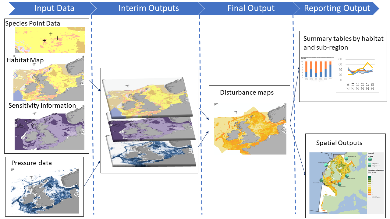
Figure 1: Interlinkage between data inputs, processes, and outputs for the BH3 indicator
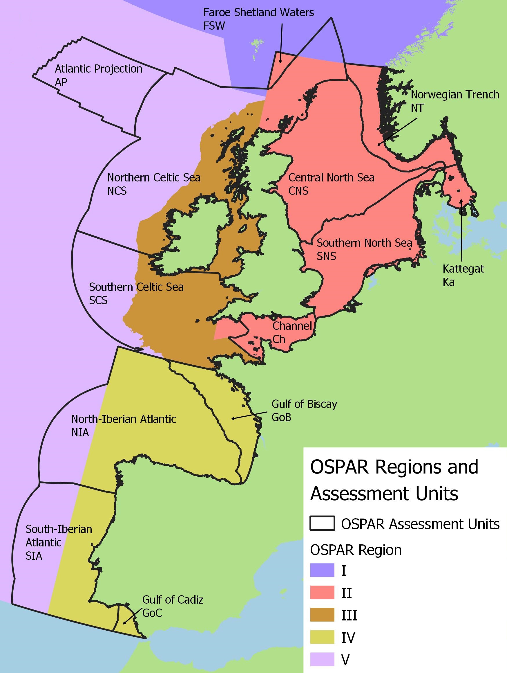
Figure 2: OSPAR assessment units used to report BH3 results against
The BH3 fisheries assessment aims to evaluate the potential risk of physical seabed disturbance caused by surface and subsurface abrasion, associated with mobile bottom-contacting fishing gears; see separate BH3b indicator assessment for extraction pressure associated with commercial aggregate extraction. Understanding of anthropogenic seafloor physical disturbance is integral to the successful delivery of ecosystem-based management to safeguard and conserve marine environments in the North-East Atlantic.
Across the OSPAR Maritime Area, shifts in benthic community composition have been reported where large and long-lived species have been replaced by small and fast-growing, opportunistic species following anthropogenic disturbance. Opportunistic species can benefit from the occurrence of physical disturbance and therefore, the subsequent availability of dead organisms following bottom-trawling events (Jennings et al., 1999; OSPAR, 2010; van Denderen et al., 2015; Serrano et al., 2022). Bottom trawling is widespread across the OSPAR Maritime Area, with potential to cause physical disturbance to a broad variety of marine species and habitats (OSPAR, 2017a). The ubiquitous distribution of fishing pressure and its coincidence with sensitive marine ecosystems highlight the imperative for improving our understanding of pressure-receptor relationships and mitigating anthropogenic impacts.
To analyse the effects human activities, such as bottom-contact fishing, can have in marine environments, understanding of the pressures they exert on marine ecosystems is required. Pressure can be defined as “the mechanism through which an activity has an effect on any part of the ecosystem”, the nature of the pressure is determined by the type of activity, intensity, and its distribution (Robinson et al., 2008). Previous studies have established an evidence base for understanding relationships between human activities and their associated pressures in marine environments via literature review (Defra, 2015; Robson et al., 2018). The two physical pressures associated with bottom-contact fishing selected for this assessment included abrasion / disturbance of the substrate on the surface of the seabed and penetration / disturbance of the substrate below the surface of the seabed (hereafter defined as ‘surface’ and ‘subsurface’ abrasion, respectively).
Physical abrasion pressures associated with mobile bottom-contacting fishing gears are categorised by métier-specific penetration depths of gear elements, dependent on whether they cause surface or subsurface abrasion (JNCC, 2011; Church et al., 2016). Surface abrasion is caused by all mobile bottom-contacting fishing gears and can adversely affect the seabed surface and upper layers of sediment (< 2 cm in depth) (ICES, 2021). Subsurface abrasion is defined as the fishing gear penetration of the substrate ≥ 2 cm below the surface (ICES, 2021). Subsurface abrasion is a component of surface abrasion and therefore, only occurs in the presence of surface abrasion, due to specific gear components that penetrate ≥ 2 cm below the seafloor surface (e.g., otter trawls doors). Abrasion pressures from mobile bottom-contacting fishing gears (surface and subsurface abrasion) can adversely affect benthic habitats and associated epifaunal and infaunal species to varying degrees, dependent on the species and habitats that are affected. Therefore, although subsurface abrasion is a subcompact of surface abrasion, it is important to consider sensitivity associated with the two pressures separately, when assessing receptor pressure-response relationships. To further understand the effect that these two pressures have on parts of the ecosystem, information quantifying fishing intensity (defined as the area swept by fishing gears per unit area) (Sanders and Morgan, 1976; ICES, 2021) is required (Eno et al., 2013; Eigaard et al., 2016; van Loon, et al., 2018).
Physical pressures can result in permanent changes to the original morphological state of the seabed. However, it is possible for biological / ecological recovery to be reached, without the recovery of physical seabed morphology (Desprez et al., 2022). Therefore, BH3 assessments primarily focus on biological communities and consider physical disturbance as potentially reversible change; BH3 does not assess the physical loss of habitats (a permanent loss of habitat through change to another substrate type). Although physical disturbance is a potentially reversable change, the degree of impact it can have on marine species and habitats depends on the biological traits of organisms, such as life history and physical structure (Collie et al., 2001; Lambert et al., 2014; van Denedren et al., 2015). Varied traits of marine species and habitats can dictate their ability to tolerate or resist change (resistance) and their ability to recover (resilience) (Tillin et al., 2010; BioConsult, 2013; Eno, et al., 2013; Lambert et al., 2014; Tillin and Tyler-Walters, 2014a & 2014b; Tyler-Walters et al., 2018). Both resistance and resilience are combined to understand sensitivity to a given pressure. If the intensity of the pressure is also known, the combination of pressure intensity and biota sensitivity can be used to assess the potential degree of physical disturbance to marine species and habitats.
Previous OSPAR assessments to understand the status of benthic habitats in the North-East Atlantic in response to human activity have been undertaken via the OSPAR Quality Status Report, 2010 (QSR 2010) and OSPAR Intermediate Assessment, 2017 (IA 2017). In the QSR 2010, there was no quantitative assessment of the extent of physical disturbance to benthic habitats, and regional assessments of fishing pressure on benthic habitats were undertaken via expert judgement only. The IA 2017 delivered the first quantitative assessment on the extent of physical disturbance to benthic habitats using Vessel Monitoring Systems (VMS) and logbook data (hereafter referred to as VMS data) to understand physical disturbance caused by bottom-contact fishing via BH3.
In the IA 2017, VMS data from 2010 to 2015 were analysed, finding that bottom-contact fishing physically disturbed 86% of the Greater North Sea and Celtic Seas, with 58% of these areas being highly disturbed (OSPAR, 2017a). Across the IA 2017 assessment period, 74% of assessed areas experienced ‘Consistent’ annual fishing pressure, which likely impacted the ability of habitats to recover. The IA 2017 assessment concluded that areas in the Celtic Seas and English Channel experienced the highest levels of disturbance. Levels of fishing pressure across the six-year assessment period fluctuated, with a quarter of assessed grid cells indicating high variability in fishing pressure. Overall, no clear trends were identified across habitats or Regions in the IA 2017 assessment (OSPAR, 2017a).
Findings are presented in two intervals: 2009 to 2020 and 2016 to 2020; corresponding to the decadal QSR assessment and the six-year period used by European Union (EU) Member States to assess progress from the second Article 8 reporting of the EU Marine Strategy Framework Directive (MSFD) in 2018, respectively. The BH3 assessment method is an agreed OSPAR Common Indicator for the Greater North Sea, the Celtic Seas and the Bay of Biscay and Iberian Coast Regions (OSPAR Regions II, III and IV; including the following marine assessment units: Faroe Shetland Waters, Central North Sea, Southern North Sea, Channel, Norwegian Trench, Kattegat, Northern Celtic Sea, Southern Celtic Sea, Gulf of Biscay, North-Iberian Atlantic, South-Iberian Atlantic, and Gulf of Cadiz). The BH3 assessment method is an OSPAR Candidate Indicator for the Atlantic Projection assessment unit, located in OSPAR Region V (Figure 2).
The OSPAR Quality Status Report 2023 (QSR 2023) assessment builds on previous analyses of physical disturbance, through the inclusion of new evidence and method improvements. Data updates comprise improved species data, habitat maps and associated sensitivity information, new aggregated bottom-contact fishing ICES VMS layers (subsequently analysed as BH3 pressure categories) and the integration of previously unassessed activities, specifically, commercial aggregate extraction (please note, assessments of bottom-contact fishing and commercial aggregate extraction are presented in separate indicator reporting templates) (Figure 1). The QSR 2023 also introduces method changes that increased accuracy when analysing sensitivity, facilitating disturbance assessments at a biotope resolution (e.g., European Nature Information System (EUNIS) Level 6), a key improvement from the IA 2017 assessment, where sensitivity assessments were limited to a broad-scale habitat resolution only (EUNIS Level 3) (Moss, 2008; OSPAR, 2017a). Assessments were undertaken using the greater resolutions of the EUNIS 2007 hierarchy (data dependent) and subsequently translated to MSFD from EUNIS for reporting purposes under the MSFD. Furthermore, the QSR 2023 uses new marine assessment units, agreed by OSPAR, facilitating integration with national reporting for Contracting Parties. The QSR 2023 assessment period ranges from 2009 to 2021. However, due to the availability of pressure data at the time of assessment, information analysed via BH3 ranged from 2009 to 2020 only.
The BH3 method comprises four main components: the creation of a composite habitat map; assessments of sensitivity; the creation of pressure layers and the calculation of potential physical disturbance. Inputs are combined using a stepwise approach to calculate the total area of potential disturbance within assessment units:
- A composite habitat map showing the extent and distribution of habitats at different scales of the EUNIS 2007 classification based on observational and modelled data. ‘Step 5: EUNIS to MSFD Benthic Broad Habitat Type (BHT) Translation’ for a detailed summary of translation process from EUNIS 2007 to MSFD BHT classification for national reporting.
- Species and habitat sensitivity, derived from resistance (ability to withstand a given pressure) and resilience (ability of a habitat to recover) (Holling, 1973; Tillin et al., 2010; BioConsult, 2013; Tillin and Tyler-Walters, 2014a & 2014b; Tyler-Walters, et al., 2018; Last et al., 2020).
- Distribution and intensity of pressures from human activities causing physical disturbance (surface abrasion, subsurface abrasion, extraction) to the seabed.
- Calculation of potential disturbance of benthic habitats, per habitat type and per assessment unit. Calculation of potential disturbance is based on the intensity of pressures and degree of habitat sensitivity per pressure type.
Step 1: Composite habitat map (not including OSPAR Threatened and / or Declining Habitats assessments)
A composite habitat map was developed to show the extent and distribution of habitats and their associated sensitivities (Castle et al., 2021). The specification for a habitat map for the assessment included the following conditions:
- To contain information on the relevant EUNIS habitat / biotope type at any level between EUNIS Levels 2 and 6;
- To refer data on biotopes to Level 3 of the EUNIS habitat classification system;
- To use the broad-scale modelled map, EUSeaMap when higher resolution maps from surveys were not available;
- To use the best available evidence on habitat data;
- To cover the greatest possible area of the OSPAR Maritime Area;
- To contain no overlaps; and
- To enable classification to Broad Benthic Habitat Types (BHT) under MSFD where possible.
The OSPAR-scale habitat map integrated component habitat maps from both in-situ survey datasets and modelled data (in the absence of direct sample data). Habitats were mapped to the highest resolution of detail available, ranging from EUNIS Level 2 (physical habitats) to Level 6 (biological communities) via the following data sources and processes:
- EUNIS habitat maps derived from surveys within the OSPAR Maritime Area extracted from EMODnet spatial data downloads portal (https://www.emodnet-seabedhabitats.eu/access-data/download-data/).
- Remaining gaps filled by EUSeaMap 2021 (Broad-scale predictive habitat maps) comprising:
- EUSeaMap 2021 obtained from EMODnet spatial data downloads portal (https://www.emodnet-seabedhabitats.eu/access-data/download-data/) (Vasquez et al., 2021) which covered all European sea basins where the EMODnet Geology seabed substrate map is available.
- UKSeaMap 2018 (Manca and Lillis, 2022) a version of EUSeaMap that incorporated greater spatial resolution data available in United Kingdom waters, as revised by the Joint Nature Conservation Committee (JNCC). UKSeaMap 2018 was incorporated to ensure the highest resolution of data was used where available.
EUSeaMap is updated every 2 to 3 years, developed using a suite of EMODnet products, including EMODnet Bathymetry, EMODnet Geology and Copernicus marine services via the Copernicus Marine Environment Monitoring Service (CMEMS) (Vasquez et al., 2021). Additional physical data used for the calculation of the models include data on light attenuation, light at the seabed and kinetic current and wave energy datasets. For further detail on associated data products, please see EMODnet (2021).
EUSeaMap data were combined with in-situ survey datasets across the OSPAR Maritime Area through two confidence-scoring mechanisms to ensure the best available data were mapped. Primarily, data were analysed for MESH (Mapping European Seabed Habitats) confidence, which assessed the quality of the processes used to create the map (e.g., maps derived from remote sensing and ground-truthing to inform habitat classification were prioritised over modelled data) (Castle et al., 2021). Subsequently, maps were reanalysed using a three-step confidence-scoring mechanism to produce a qualitative score, indicative of the likelihood of habitats being mapped correctly within a study area (please see Ellwood, (2014) for full detail of the three-step confidence assessment):
- Remote sensing coverage
- Amount of sampling
- Distinctness of class boundaries
To ensure that the OSPAR-scale composite habitat map met the above conditions, the following quality controls were applied to all source data prior to use:
- Restricted and public data were identified; only publicly available data were considered in analyses.
- Mosaic habitats were formatted using the same schema as the previous combined map.
All data included were also quality checked using a five-stage stepwise method to resolve GIS errors and overlapping habitat polygons to ensure that the most accurate polygon was represented in final map outputs. An overview of the five stages is represented below:
- If one layer contained all intertidal habitats and another layer contained all subtidal habitats, the layer containing all intertidal habitats was used. A prioritisation of layers containing intertidal habitats was undertaken, as intertidal maps were generally produced with better detail and resolution than subtidal data and therefore, had better accuracy. Where both layers contained all intertidal or all subtidal habitats, or either layer contained a mixture of intertidal and subtidal habitats, stage 2 was implemented.
- The layer with the highest 3-step confidence score was used, where the 3-step confidence score was the same, stage 3 was implemented.
- The layer derived from survey data was prioritised over modelled data derived from EUSeaMap; where both layers were based on survey data, stage 4 was implemented.
- The layer with the highest MESH confidence score was used; where both layers shared the same MESH confidence score, stage 5 was implemented.
- Expert judgement on the most likely layer to indicate EUNIS Level 3 habitat was applied, and that layer was used.
This process was repeated until all overlapping polygons had been resolved within the layer. Once overlapping polygons had been resolved to represent the habitat most likely present in the area, a ‘Repair Geometry’ tool was used to resolve any geometry errors in the OSPAR-scale composite habitat map.
Step 2: Assessing Sensitivity
Step 2 of the assessment involved creating a sensitivity layer that quantified the sensitivity of species and habitats within the OSPAR Maritime Area to surface and subsurface abrasion pressures separately. Habitat polygon data used in the sensitivity assessment were obtained from the analyses previously described in ‘Step 1’. Sampled in-situ species point data were compiled from the OSPAR QSR Data Call in 2021, UK Marine Recorder (Public) snapshot (version "2022-01-24"), and from data submitted directly by OSPAR Contracting Parties. In some instances, data were provided with start and end trawl locations, these data were assigned a midpoint for the in-situ species records. To align biological records with the QSR assessment period, sample data were only included from 2009 onwards.
Sensitivity information used in the assessment included Marine Evidence based Sensitivity Assessments (MarESA) and Defra MB0102 Report No. 22, Task 3: Development of a Sensitivity Matrix (pressures-MCZ / MPA features) (hereafter referred to as MB0102) (Tillin et al., 2010; Tyler-Walters et al., 2018). The aforementioned sensitivity assessments were not site-specific and were based on the likely effects of a pressure in the centre of the distributional range of a habitat or species (Tyler-Walters et al., 2018). Several factors associated with the specific location of habitats and species, such as the underlying substratum, can affect their sensitivity to specific pressures (Tyler-Walters et al., 2018). Therefore, additional sources of habitat and species sensitivity assessments were investigated for incorporation into the BH3 method, including Sentinels of Seabed (SoS) indicator (Serrano et al., 2022) and Condition of benthic habitat communities (OSPAR, 2018). These additional sources showed potential to broaden the evidence base with the inclusion of regional VMS pressure-response assessments (Regions II and IV). However, alignment of these additional assessments with the BH3 method was not possible within the QSR reporting period and will be explored in future work. Species sensitivity values were assigned to species records that Contracting Parties had confirmed occurred in their waters (where data were provided).
MarESA is a scientific approach to assessing sensitivity of habitats (including habitat characterising species) within the North-East Atlantic to a range of pressures, based on those defined by the OSPAR Intercessional Correspondence Group on Cumulative Effects (ICG-C) (OSPAR, 2011 & 2014; Tyler-Walters et al., 2018). MB0102 was a Defra funded project completed to support the designation of Marine Conservation Zone MPAs under the Marine and Coastal Access Act in the United Kingdom. Outputs of the project included sensitivity assessments for designated MPA features, EUNIS Level 3 broad-scale habitats and OSPAR Threatened and / or Declining Habitats to pressures in the marine environment, alongside associated pressure benchmarks (Tillin et al., 2010).
When developing BH3 sensitivity layers, MarESA was prioritised over MB0102 sensitivity due to improved data quality and accuracy; MB0102 relied on expert judgement, whereas MarESA assessments were literature-based, peer-reviewed publications that included detailed evaluations of evidence used to inform assessments and audit trails (Tyler-Walters et al., 2018). Evidence used to inform MarESA assessments were representative of organisms and biotopes, including their known ranges and distributions, in response to specific pressures. Evidence was prioritised based on its relevance to assessed features; for example, evidence from the North-East Atlantic was prioritised over literature and studies from elsewhere when assessing organisms found in the North-East Atlantic. In addition, MarESA sensitivity assessments underwent quality assurance checks by the Marine Life Information Network (MarLIN) Editor and were peer reviewed by one or more independent expert(s) (Tyler-Walters, et al., 2018). Therefore, MB0102 sensitivity information was only used in instances where species or habitat records did not have completed MarESA sensitivity assessments.
In MB0102, species that characterised sublittoral rock and sediment habitats were assessed for their sensitivity to pressures in groups of taxa with similar biological traits. The resistance and resilience of characteristic species were assessed in response to defined pressures via literature review and expert judgement. Please see Tillin and Walters (2014a), Tillin and Walters (2014b), Maher and Alexander (2016) and Maher et al., (2016) for details of habitat characterising species, trait-based groupings, sensitivity assessments and assessment confidence scores.
In both MB0102 and MarESA sensitivity assessments, the following component information were considered (see Tillin & Tyler-Walters 2014a & 2014b; Maher and Alexander, 2016; Tyler-Walters et al., 2018 for further detail of methods):
- Establish and define the key components of the assessed feature, considered relevant to the assessment (e.g., traits such as life history and the ecology of the key and characterising species). Only species naturally found in the absence of pressures were selected for the sensitivity assessments (Table a).
- Assess the resistance and resilience of the feature to a defined pressure; scales of assessment for resistance and resilience are given in Table b and Table c, respectively.
| Key structural species | The species provides a distinct habitat that supports an associated community. Loss/degradation of this species population would result in loss/degradation of the associated community. |
|---|---|
| Key functional species | Species that maintain community structure and function through interactions with other members of that community (for example through predation, or grazing). Loss/degradation of this species population would result in rapid, cascading changes in the community. |
| Important characteristic species | Species characteristic of the biotope (dominant, and frequent) and important for the classification of the habitat. Loss/degradation of these species populations may result in changes in habitat classification. |
| Resistance | Description |
|---|---|
| None | Key functional, structural, characterizing species severely decline and/or physicochemical parameters are also affected e.g., removal of habitats causing a change in habitats type. A severe decline/reduction relates to the loss of 75% of the extent, density or abundance of the selected species or habitat component e.g., loss of 75% substratum (where this can be sensibly applied). |
| Low | Significant mortality of key and characterizing species with some effects on the physicochemical character of habitat. A significant decline/reduction relates to the loss of 25-75% of the extent, density, or abundance of the selected species or habitat component e.g., loss of 25-75% of the substratum. |
| Medium | Some mortality of species (can be significant where these are not keystone structural/functional and characterizing species) without change to habitats relates to the loss <25% of the species or habitat component. |
| High | No significant effects on the physicochemical character of habitat and no effect on population viability of key/characterizing species but may affect feeding, respiration, and reproduction rates. |
| Resilience | Description |
|---|---|
| Very Low | Negligible or prolonged recovery possible; at least 25 years to recover structure and function |
| Low | Full recovery within 10-25 years |
| Medium | Full recovery within 2-10 years |
| High | Full recovery within 2 years |
- Combine resistance and resilience to derive a BH3 sensitivity score to a defined pressure via the BH3 sensitivity matrix. The BH3-specific sensitivity matrix was derived from the IA 2017, presenting combined resistance and resilience scores as a single sensitivity value (ranging from 1 to 5, with 5 being the most sensitive; Table d).
Table d: Sensitivity matrix combining resistance and resilience scores to produce a sensitivity score ranging from 1 to 5, where 5 is the most sensitive.
| Sensitivity | Resilience | |||||
| very low (>25 yr.) | low (>10-25 yr.) | medium (>2-10 yr.) | high (1-2 yr.) | very high (<1 yr.) | ||
| Resistance | none | 5 | 4 | 4 | 3 | 2 |
| low | 4 | 4 | 3 | 3 | 2 | |
| medium | 4 | 3 | 3 | 2 | 1 | |
| high | 3 | 3 | 2 | 2 | 1 | |
Both MarESA and MB0102 contain assessments for a range of pressure benchmarks (e.g., descriptors of the pressure: magnitude, extent, duration, and frequency of the effect) specific to assessed human activities. Therefore, to ensure that appropriate assessments were used with specific activities, established pressure-activity relationships were identified via literature review and the JNCC Marine Pressures-Activities Database, Version 1.5 (Robson et al., 2018). Two pressures known to cause physical disturbance associated with bottom-contact fishing were selected (Table e) and relevant sensitivity assessments were used from MarESA and MB0102. Sensitivity values to both surface and subsurface abrasion pressures were assigned to species and habitats, where available, to enable independent assessment of risk of disturbance from both pressures. However, the method of combining both species and habitat sensitivity described below was the same for both surface and subsurface sensitivity scores.
| OSPAR ICG-C Pressure | Assessment benchmark | Definition |
|---|---|---|
| Abrasion/disturbance at the surface of the substratum | Benthic species /habitats: damage to surface features (e.g., species and physical structures within the habitat) | Physical disturbance or abrasion at the surface of the substratum in sedimentary or rocky habitats. The effects are relevant to epiflora and epifauna living on the surface of the substratum. In intertidal and sublittoral fringe habitats, surface abrasion is likely to result from recreational access and trampling (inc. climbing) by human or livestock, vehicular access, moorings (ropes, chains), activities that increase scour and grounding of vessels (deliberate or accidental). In the sublittoral, surface abrasion is likely to result from pots or creels, cables and chains associated with fixed gears and moorings, anchoring of recreational vessels, objects placed on the seabed such as the legs of jack-up barges, and harvesting of seaweeds (e.g., kelps) or other intertidal species (trampling) or of epifaunal species (e.g., oysters). In sublittoral habitats, passing bottom gear (e.g., rock hopper gear) may also cause surface abrasion to epifaunal and epifloral communities, including epifaunal biogenic reef communities. Activities associated with surface abrasion can cover relatively large spatial areas e.g., bottom trawls or bio-prospecting or be relatively localized activities e.g., seaweed harvesting, recreation, potting, and aquaculture. |
| Penetration and/or disturbance of the substratum below the surface | Benthic species /habitats: damage to sub-surface features (e.g., species and physical structures within the habitat) | Physical disturbance of sediments where there is limited or no loss of substratum from the system. This pressure is associated with activities such as anchoring, taking of sediment/geological cores, cone penetration tests, cable burial (ploughing or jetting), propeller wash from vessels, certain fishing activities, e.g., scallop dredging, beam trawling. Agitation dredging, where sediments are deliberately disturbed by and by gravity & hydraulic dredging where sediments are deliberately disturbed and moved by currents could also be associated with this pressure type. Compression of sediments, e.g., from the legs of a jack-up barge could also fit into this pressure type. Abrasion relates to the damage of the seabed surface layers (typically up to 50 cm depth). Activities associated with abrasion can cover relatively large spatial areas and include fishing with towed demersal trawls (fish & shellfish); bio-prospecting such as harvesting of biogenic features such as maerl beds where, after extraction, conditions for recolonization remain suitable or relatively localised activities including seaweed harvesting, recreation, potting, aquaculture. Change from gravel to silt substrata would adversely affect herring spawning grounds. Loss, removal, or modification of the substratum is not included within this pressure (see the physical loss pressure theme). Penetration and damage to the soft rock substrata are considered, however, penetration into hard bedrock is deemed unlikely. |
Assigning sensitivity to habitats: MarESA habitat sensitivity assessments were available for a diversity of biotopes, ranging from Level 4 to 6 of the EUNIS classification, complete with detailed evaluations and audit trails of the information used to assess sensitivity (Tyler-Walters, 2018; Last et al., 2020). Although MarESA assessments enabled detailed biotope-resolution sensitivity and disturbance assessments, high-resolution EUNIS habitat data were not available throughout the entire OSPAR Maritime Area. Wherever possible, biotope-scale assessments were used in disturbance calculations (e.g., EUNIS Levels 4, 5 and 6). Due to data paucity, sensitivity assessments were not available at all resolutions of the EUNIS hierarchy associated with habitat map polygons; particularly, when mapping at a broadscale-habitat level (e.g., EUNIS Levels 2 and 3). Therefore, automated methods based on the JNCC MarESA Aggregation were developed in Python 3.6 (Python Software Foundation, 2020), to aggregate biotope-resolution resistance and resilience data to higher hierarchical tiers of the EUNIS classification (Last et al., 2020). Aggregation of resistance and resilience values were undertaken independently across EUNIS tiers to enable child biotope resistance and resilience values to be assigned to parent biotopes, on a precautionary basis to return the lowest respective resistance and resilience values to assessed pressures (please see example given in Table f). Aggregated resistance and resilience values were subsequently converted to sensitivity scores using the aforementioned BH3 sensitivity matrix (Table d) to obtain the most precautionary sensitivity value derived from child biotopes. For further detail on the aggregation methods, see Last et al., (2020). To maximise available data coverage, MB0102 sensitivity assessments (resistance and resilience) were used for habitats that did not have MarESA assessments (e.g., not assessed, or sensitivity not available for the assessed pressures). In instances where multiple MB0102 sensitivity scores were available for the same EUNIS code, scores with the highest confidence were assigned; if both confidence assessments were equal, then the most precautionary values were used.
| EUNIS Level 3 | Level 3 Resistance | EUNIS Level 4 | Level 4 Resistance | EUNIS Level 5 | Level 5 Resistance Range | EUNIS Level 6 | Level 6 Resistance Range |
|---|---|---|---|---|---|---|---|
| A5.4 (None) | Medium, Low, None | A5.41 (Unknown) | Unknown | A5.411 | Unknown | No child biotopes | |
| A5.412 | Unknown | ||||||
| A5.42 (Low) | Low | A5.421 | Low | ||||
| A5.422 | Low | ||||||
| A5.43 (None) | Medium, Low, None | A5.431 | Low | ||||
| A5.432 | Low | ||||||
| A5.433 | Medium | ||||||
| A5.434 | None | ||||||
| A5.435 | Low | ||||||
| A5.44 (Low) | Medium, Low | A5.441 | Medium | A5.4411 | Medium | ||
| A5.442 | Low | No child biotopes | |||||
| A5.443 | Medium | ||||||
| A5.444 | Low | ||||||
| A5.445 | Low | ||||||
| A5.446 | Unknown | ||||||
| A5.45 (Medium) | Medium | A5.451 | Medium | ||||
| A5.46 (Unknown) | Unknown | A5.461 | Unknown | ||||
| A5.462 | Unknown | ||||||
| A5.463 | Unknown | ||||||
| A5.47 (Unknown) | Unknown | A5.471 | Unknown | ||||
| A5.472 | Unknown | ||||||
Assigning sensitivity to species:
Species-specific resistance and resilience scores from MarESA and MB0102 were combined to maximise data coverage, increasing the total number of species with associated sensitivity assessments (Table g). Species-specific resistance and resilience scores for the associated pressures were combined into a single sensitivity score using the same process described for habitat sensitivity (Table d).
| Species | BH3 Sensitivity | Sensitivity assessment source | |
|---|---|---|---|
| Abrasion/disturbance of the substrate on the surface of the seabed | Penetration and/or disturbance of the substrate below the surface of the seabed, including abrasion | ||
| Abra alba | 2 | 2 | Sediment |
| Abra nitida | 3 | 3 | Sediment |
| Abra prismatica | 3 | 3 | Sediment |
| Alcyonium digitatum | 3 | 3 | Sediment; Sublittoral rock |
| Alkmaria romijni | 3 | 3 | MarESA |
| Ampharete falcata | 3 | 3 | Sediment |
| Amphianthus dohrnii | 3 | Not Assessed | MarESA |
| Amphiura filiformis | 3 | 3 | Sediment |
| Arctica islandica | 4 | 4 | MarESA |
| Ascidiella aspersa | 3 | 3 | Sediment |
| Asterias rubens | 2 | 3 | Sediment; Sublittoral rock |
| Astropecten irregularis | 3 | 3 | Sediment |
| Atrina fragilis | 3 | 5 | MarESA |
| Axinella dissimilis | 3 | Not Assessed | Sublittoral rock |
| Balanus crenatus | 3 | 3 | Sediment |
| Bathyporeia elegans | 2 | 2 | Sediment |
| Branchiostoma lanceolatum | 3 | 3 | Sediment |
| Brissopsis lyrifera | 2 | 3 | Sediment |
| Caecum armoricum | 3 | 5 | MarESA |
| Calocaris macandreae | 3 | 4 | Sediment |
| Calvadosia campanulata | 3 | 5 | MarESA |
| Calvadosia cruxmelitensis | 3 | 4 | MarESA |
| Cancer pagurus | 2 | No Information | Sublittoral rock |
| Cerianthus lloydii | 3 | 3 | Sediment |
| Chaetozone zetlandica | 3 | 3 | Sediment |
| Cladophora rupestris | 2 | Not Assessed | Sublittoral rock |
| Clavelina lepadiformis | 3 | Not Assessed | Sublittoral rock |
| Cliona celata | 2 | Not Assessed | Sublittoral rock |
| Dipolydora caulleryi | 2 | 3 | Sediment |
| Dysidea fragilis | 3 | Not Assessed | Sublittoral rock |
| Echinocardium cordatum | 2 | 3 | Sediment |
| Echinocyamus pusillus | 2 | 3 | Sediment |
| Echinus esculentus | 3 | 3 | Sediment; Sublittoral rock |
| Electra pilosa | 3 | Not Assessed | Sublittoral rock |
| Eudorellopsis deformis | 2 | 3 | Sediment |
| Eunicella verrucosa | 3 | Not Assessed | MarESA |
| Flustra foliacea | 2 | 3 | Sediment; Sublittoral rock |
| Funiculina quadrangularis | 4 | 4 | Sediment |
| Gammarus insensibilis | 3 | Not Assessed | MarESA |
| Glycera lapidum | 2 | 3 | Sediment |
| Haliclystus auricula | 3 | 4 | MarESA |
| Halidrys siliquosa | 2 | Not Assessed | Sublittoral rock |
| Hippocampus hippocampus | 3 | 3 | MarESA |
| Iphinoe trispinosa | 2 | 3 | Sediment |
| Laminaria hyperborea | 2 | Not Assessed | Sublittoral rock |
| Lanice conchilega | 2 | 2 | Sediment; Sublittoral rock |
| Lithothamnion corallioides | 5 | 5 | MarESA |
| Maxmuelleria lankesteri | 3 | 3 | Sediment |
| Modiolus modiolus | 4 | 4 | Sediment |
| Mytilus edulis | 2 | No Information | Sublittoral rock |
| Nematostella vectensis | 2 | 2 | MarESA |
| Nemertesia ramosa | 3 | 3 | Sediment |
| Neopentadactyla mixta | 2 | 3 | Sediment |
| Nephrops norvegicus | 3 | 3 | Sediment |
| Nephtys hombergii | 2 | 2 | Sediment |
| Nucella lapillus | 2 | No Information | Sublittoral rock |
| Obelia longissima | 3 | 3 | Sediment |
| Ophiocomina nigra | 3 | 3 | Sediment |
| Ophiothrix fragilis | 3 | 3 | Sediment |
| Ophiura albida | 3 | 3 | Sediment |
| Ostrea edulis | 4 | 4 | MarESA |
| Padina pavonica | 2 | Not Assessed | MarESA |
| Pagurus bernhardus | 3 | 3 | Sediment |
| Palinurus elephas | 3 | Not Assessed | MarESA |
| Palmaria palmata | 2 | Not Assessed | Sublittoral rock |
| Paramphinome jeffreysii | 2 | 3 | Sediment |
| Pecten maximus | 3 | 3 | Sediment |
| Pennatula phosphorea | 3 | 3 | Sediment |
| Phaxas pellucidus | 3 | 3 | Sediment |
| Pholas dactylus | 2 | No Information | Sublittoral rock |
| Phymatolithon calcareum | 5 | 5 | MarESA |
| Polydora ciliata | 2 | No Information | Sublittoral rock |
| Protodorvillea kefersteini | 2 | 2 | Sediment |
| Sabella pavonina | 2 | No Information | Sublittoral rock |
| Scoloplos armiger | 2 | 2 | Sediment |
| Sepia officinalis | 3 | 3 | MarESA |
| Sertularia argentea | 3 | 3 | Sediment |
| Spirobranchus triqueter | 3 | Not Assessed | Sediment; Sublittoral rock |
| Styela gelatinosa | 3 | 3 | Sediment; Sublittoral rock |
| Thyasira flexuosa | 3 | 3 | Sediment |
| Timoclea ovata | 3 | 3 | Sediment |
| Urticina felina | 3 | 3 | Sediment |
| Virgularia mirabilis | 3 | 3 | Sediment |
Creating a final sensitivity layer using both habitat and species sensitivity data:
Once habitat and species sensitivity data were assigned to the composite habitat map and the species point data respectively, the sensitivity map used in the BH3 assessment was created using the following stages:
- Stage one: The composite habitat map, with associated habitat sensitivity values added, was spatially intersected in ESRI ArcGIS v10.1 with a 0,05° x 0,05° grid (spatially aligned with ICES c-squares) to create a gridded habitat sensitivity layer. This grid resolution was chosen to align with the resolution of the VMS pressure data.
- Stage two: The in-situ species points records were spatially joined to individual habitat polygons within a 0,05° x 0,05° c-squares to create a polygon layer with both habitat and, where available, species sensitivity values; note that species points were only joined to the portion of a habitat polygon that intersected the c-square the species point was located in. In instances where multiple species points overlapped a single habitat polygon within a 0,05° x 0,05° grid cell, only the maximum species sensitivity value was joined. Assigning the maximum species sensitivity followed the precautionary principle, which aimed to avoid assigning sensitivity based on the presence of less sensitive opportunistic species that can occur in high abundances in areas that have already been impacted by human activities.
- Stage three: Where in-situ species sensitivity was present the maximum value between the habitat and species sensitivity was assigned as the final sensitivity value. This maintained the precautionary approach aimed to mitigate the use of potentially less sensitive, opportunistic species, to represent an already impacted area. If species sensitivity was higher, and therefore, prioritised over habitat sensitivity, the species sensitivity value was only assigned to the portion of the polygon within the c-square where the record was observed to maximise representativity.
- Stage four: Sensitivity data were intersected and spatially joined with OSPAR assessment units. Joining sensitivity data with assessment unit polygons allowed for the quantification of area without EUNIS habitat information and therefore, area without sensitivity assessments to be analysed as unassessed disturbance when intersected with pressure data.
Step 3: Assessing the Extent and Distribution of Potential Physical Disturbance Pressures
Data overview
Step 3 of the QSR 2023 BH3 assessment involved creating a single layer that quantified annual and aggregated surface and subsurface abrasion pressure for the two assessment periods (2009 to 2020 for QSR and 2016 to 2020 for MSFD). Fishing pressure data ranging from 2009 to 2020 (2020 being the most recent data at the time of this assessment) were obtained from ICES (ICES, 2021). Data were obtained from ICES via an OSPAR data call, collating VMS and logbook data from ICES member countries to develop spatial data layers representative of fishing intensity / pressure within the OSPAR Maritime Area (ICES, 2021). Between 2009 and December 31st, 2011, VMS data were only available for fishing vessels greater than 15 m in length; following changes in the Common Fisheries Policy (EU Council Regulation No. 44 / 2012), from January 1st, 2012, onward, datasets contained VMS records from vessels over 12m in length.
The ICES data layers contained the total annual swept-area and swept-area ratio (SAR) values for both surface (< 2 cm penetration depth of the gear components) and subsurface (≥ 2 cm penetration depth of the gear components) fishing pressure. Both swept area and SAR were calculated using standardised grids, known as c-squares (0,05° x 0,05° grid cell), the spatial resolution adopted by ICES (ICES, 2021). Swept-area is a multiplication of the width of the gear in contact with the seabed by the average vessel speed and the time fished per unit area (c-square) per year. The SAR (representative of fishing intensity) is the swept-area divided by the total area of the c-square.
To ensure that assessments were representative of the actual fishing gears in contact with the seafloor, estimates of total annual surface and subsurface SAR values within each c-square were informed by parameters (e.g., gear width) associated with relevant bottom-contacting métiers (Eigaard et al., 2016; Church et al., 2016; ICES, 2021). A métier refers to a group of fishing operations targeting a specific assemblage of species, using a specific gear, during a precise period of the year and / or within the specific area (Deporte et al., 2012). For further method details on the creation of the fishing pressure layers, refer to ICES (2021).
When analysing the ICES VMS data available for the QSR 2023 assessment the following caveats should be noted:
- The data assumed fishing activity to be homogeneous over each c-square, which may have underestimated fishing intensity and overestimated fishing distribution, should fishing have been constrained to discrete areas within the c-square.
- VMS data for vessels less than 12 m in length were not available at the time of assessment. Therefore, inshore areas, or areas where vessels below 12 m in length operate may be poorly represented.
- VMS data from Portugal, Iceland and Norway were not included in assessments as the submitted data did not pass ICES quality checks, therefore, some fleet activities may be absent and / or underrepresented.
- Fishing pressure intensity (SAR, swept-area ratio) depended on the spatial resolution of the fishing pressure data (0,05° × 0,05° grid cells in this instance). It should be noted that due to the curvature of the Earth, not all c-squares had the same area in km2.
- VMS data supplied for the OSPAR Maritime Area did not include the entirety of the Kattegat assessment unit (Isse Fjord and Roskilde Fjord areas).
Analysis of fishing pressure for individual years:
Annual assessments of bottom-contact fishing pressure were conducted on categorised surface and subsurface SAR values. Categories were based on an intensity scale, ranging from ‘none’ to ‘very high’ where a cell has been swept more than 300% or three times per year (Table h). The intensity scale was developed from peer reviewed literature on the impacts of bottom trawling on benthic ecosystems, and the scale was proposed and agreed within the OSPAR Benthic Habitats Expert Group (OSPAR, 2017b).
Surface and subsurface SAR data were categorised separately using the pressure intensity scale outlined in Table h to enable independent assessment of the two separate pressures; both pressures, although spatially linked, were not considered additively, synergistically, or cumulatively. The results of Schroeder et al., (2008) indicated that a SAR of 1 was considered to have a high impact on species abundance. However, SAR values between 0 and 1 were split into three categories based on the results of calculations of van Loon (2018), suggesting a significant biological response between SAR values of 0,15 to 1. Furthermore, areas that were fished more than three times per year did not show any further levels of degradation (van Loon et al., 2018), which informed the upper limit of the pressure intensity scale (SAR >3).
As SAR values of up to 98 were observed in the ICES VMS data, and van Loon et al., (2018) indicated further degradation was not evident beyond three sweeps per year, the intensity scale used allowed for differentiation in lower SAR values, where the greatest impact on benthic ecosystems was observed. Future assessments aim to further improve the BH3 method through changes to how pressure is analysed as new evidence becomes available.
Table h: Classification of the swept area ratios per grid cell per year
| BH3 Category | SAR |
| None (0) | 0,00 |
| Very Low (1) | <0.00 - ≤0,33 |
| Low (2) | >0,33 - ≤0,66 |
| Medium (3) | >0,66 - ≤1,00 |
| High (4) | >1,00 - ≤3,00 |
| Very High (5) | >3,00 |
Analyses of fishing pressure across assessment cycles (2009 to 2020; 2016 to 2020)
To assess fishing pressure over the QSR 2023 assessment period, aggregated pressure layers were created, combining annual pressure layers into a single dataset for use in disturbance assessments using a spatial union via Geographic Information Systems (GIS) software.
When combining all annual layers via spatial unions in GIS, there were instances where c-squares had no reported VMS data for specific years in the time series. Therefore, when calculating aggregated SAR values, c-squares without reported VMS were treated as having ‘no data’, rather than 0 SAR, due to the presence of true 0 values in the annual layers before aggregation. Additionally, it was likely that although certain c-squares had no VMS data reported in select years, they were in areas suitable for bottom contact fishing. Therefore, due to the aforementioned data caveats (e.g., no reported VMS for vessels < 12 m and missing fleet data) it would have been inaccurate to assign 0 SAR values in the absence of actual reported 0 pressure. See BH3 Aggregated Pressure Map R script for full details.
The method for assessing temporal fishing variability, as agreed by OSPAR in the IA 2017 was implemented in the QSR 2023. The range of SAR categories observed across the time series was calculated for each c-square, indicating distinction between areas where fishing intensity was at ‘Consistent’ levels across years, from those where fishing intensity levels fluctuated. C-squares were considered ‘Variable’ if a range of three or more SAR categories was observed throughout the time series. The use of three or more SAR categories to denote variance originated in the IA 2017 and was based on expert judgement. C-squares that had a variance range of three or more SAR categories were used to indicate areas of opportunistic fishing, potentially new areas being explored for fishing or areas which were not used consistently.
To produce a layer showing the aggregated surface and subsurface pressures that accounted for variations in fishing pressure across years, the following method was used:
- For cells with low variability (i.e., a range of less than three SAR categories), the mean of SAR values across all years with available data was calculated (areas without SAR reported were not included in the calculation of mean SAR).
- For cells with high variability (i.e., range of three or more reported SAR categories), the highest SAR value across all years was selected following a precautionary approach to represent the most damaging levels of fishing to benthic habitats (OSPAR, 2017).
Note the mean and maximum SAR values were taken from the raw values in the ICES data (prior to intensity categorisation). The mean and maximum SAR values were then recategorised into the intensity scale (Table h) to give aggregated pressure categories for each c-square.
Step 4: Calculation of disturbance
Step 4 of the QSR 2023 BH3 assessment involved creating a spatial layer that quantified disturbance to species and habitats within the OSPAR Maritime Area. Sensitivity (outputs of Step 2) and pressure (outputs of Step 3) maps were spatially intersected via Environmental Systems Research Institute (ESRI) ArcGIS software (ESRI, 2012). Potential surface and subsurface disturbance values were calculated separately on the intersect output layer by combining surface and subsurface sensitivity with surface and subsurface pressure values, respectively, via a matrix (Table i). The matrix produced 10 categories of disturbance ranging from 0 to 9, where 9 was the maximum risk of disturbance possible. The disturbance matrix was created from previous studies that analysed the impacts of pressures on sensitive species and habitats when applied at different intensities (Schroeder et al., 2008; Rondinini, 2010; BioConsult, 2013; van Loon et al., 2018). In instances where pressure data intersected areas without sensitivity information (due to a lack of EUNIS habitat data or sensitivity assessments), outputs were classified as ‘Unassessed Disturbance’. Areas with no reported VMS data throughout the assessment period (2009 to 2020 or 2016 to 2020) were categorised as ‘Zero’ disturbance as it was deemed unlikely that fishing had occurred in these areas.
Table i: Disturbance matrix combining pressure and habitat sensitivity. Note ‘zero’ = No reported VMS data or 0 SAR value reported by ICES for vessels >12 m only
| Disturbance Matrix | Sensitivity | |||||
|---|---|---|---|---|---|---|
| 1 | 2 | 3 | 4 | 5 | ||
| Pressure | Null / 0 | 0 | 0 | 0 | 0 | 0 |
| 1 | 1 | 2 | 3 | 4 | 6 | |
| 2 | 1 | 2 | 4 | 6 | 7 | |
| 3 | 1 | 3 | 5 | 7 | 9 | |
| 4 | 1 | 4 | 6 | 8 | 9 | |
| 5 | 2 | 4 | 7 | 9 | 9 | |
Annual and aggregated (2009 to 2020; 2016 to 2020 assessment periods) potential surface and subsurface disturbance values were calculated separately from the corresponding annual and aggregated pressure categories. The maximum disturbance category, between surface and subsurface disturbance, for each habitat polygon within a c-square was presented as the final disturbance category for each assessment period, following a precautionary principle.
For reporting purposes, disturbance categories were summarised into four groups (‘Zero’ = no reported VMS data or 0 SAR, ‘Low’ = disturbance categories 1 to 4, ‘Moderate’ = disturbance categories 5 to 7, and ‘High’ = disturbance categories 8 and 9) derived from the 0-9 disturbance scale (Table j) (Schroeder et al., 2008; OSPAR, 2017). Groups were chosen to summarise the pressure and sensitivity elements of the physical disturbance values. Areas considered to have ‘low’ (1 to 2) or ‘moderate’ (3) sensitivity were not represented in the ‘High’ disturbance group. Pressure values of 3 and greater than 3 in higher sensitivity areas (4 and 5 respectively) accounts for all ‘High’ disturbance. Areas with pressure values less than 3 were not included in the ‘High’ disturbance group. Please note, these groupings are not representative of thresholds and should be used for comparative interpretations of disturbance outputs across the OSPAR Maritime Area only.
Table j: Disturbance matrix with summary groups; ‘Low’ (1-4), ‘Moderate’ (5-7), and ‘High’ (8-9). Note ‘Null / 0*’ pressure = No reported VMS data or 0 SAR value reported by ICES for vessels >12 m only
| Disturbance Matrix | Sensitivity | |||||
|---|---|---|---|---|---|---|
| 1 | 2 | 3 | 4 | 5 | ||
| Pressure | Null / 0 | 0 | 0 | 0 | 0 | 0 |
| 1 | 1 | 2 | 3 | 4 | 6 | |
| 2 | 1 | 2 | 4 | 6 | 7 | |
| 3 | 1 | 3 | 5 | 7 | 9 | |
| 4 | 1 | 4 | 6 | 8 | 9 | |
| 5 | 2 | 4 | 7 | 9 | 9 | |
Following consultation and review via national experts within the OSPAR framework, areas where draft disturbance outputs were considered erroneous were identified. Within the Norwegian Trench and the Kattegat, the Trålgräns and Fredingsområde Södra, ‘No Trawl Zones’ (hereafter referred to as Swedish No Trawl Zone), were identified as areas where trawling was known to be absent between the 2009 to 2020 assessment period. Spatial disturbance outputs in the Kattegat and Norwegian Trench were, therefore, intersected with the boundary of the Swedish No Trawl Zone provided by national experts. Areas within the Swedish No Trawl Zone were subsequently amended to disturbance group ‘Zero’, regardless of reported VMS data, to ensure established fisheries management measures were accurately represented. The size of available c-square grid cells and assumed homogeneity of SAR values likely resulted in the erroneous allocation of fishing pressure in areas with established fisheries management measures.
In addition to the Swedish No Trawl Zone, areas of deep-sea habitat in the North-Iberian Atlantic contained reported bottom-contacting fishing pressure in locations considered too deep for bottom trawling. National experts highlighted that the presence of VMS data with SAR values in such areas were likely due to vessel speeds slowing for bad weather when in transit across the Bay of Biscay, rather than true fishing activity. Therefore, disturbance values within the Atlantic lower abyssal and Atlantic mid abyssal biological zones (derived from EUSeaMap2021) were amended to disturbance group ‘Zero’ within the assessment unit, due to high confidence that bottom trawling would not happen in such deep areas of the North-Iberian Atlantic. Conversely, concentrated areas of disturbance recorded in the Atlantic upper abyssal biological zone, around the continental shelf edge, were deemed to be potential fishing activity and therefore, not omitted from analyses.
Step 5: EUNIS to MSFD Benthic Broad Habitat Type (BHT) Translation
To maximise usability of assessment results for Contracting Parties that report against Article 8 of the MSFD, Step 5 assigned spatial outputs based on EUNIS habitat codes to the appropriate BHT in the MSFD classification system. A translation table was created by habitat classification experts at JNCC and EMODnet to facilitate correlation between the EUNIS 2007 habitat classification and BHTs. In some instances, translations required combinations of EUNIS code, biological zone and / or substrate information to correctly assign BHT where EUNIS habitats contained or partially overlapped with multiple BHTs. Biological zone and substrate information was obtained from a spatial intersect of the BH3 disturbance layer with EUSeaMap2021 (Vasquez et al., 2021) using ArcGIS v.10.1. EUNIS habitats that could not be assigned MSFD BHT translations (e.g., lacking substrate information) were designated “No EUNIS to BHT translation”.
Step 6: Assessment of OSPAR Threatened and / or Declining Habitats
Disturbance from bottom contacting fishing in OSPAR Threatened and / or Declining Habitats (OSPAR, 2008 & 2019) was assessed using the OSPAR Habitats in the North-East Atlantic Ocean - 2020 Polygons layer available from the EMODnet spatial data downloads facility [https://www.emodnet-seabedhabitats.eu/access-data/download-data/] (EMODnet, 2020). The layer is a compilation of OSPAR Threatened and / or Declining Habitats data submitted by OSPAR Contracting Parties and is a separate data product to the composite habitat map. Sensitivity of habitats were assigned using EUNIS codes included in the habitat definition and corresponding MarESA sensitivity assessments. In instances where habitats had multiple biotope codes, the maximum sensitivity was assigned following a precautionary approach.
For habitats without MarESA assessments (e.g., carbonate mounds, coral gardens, and seamounts) sensitivity was assigned following Tillin & Tyler-Walters (2010; coral carbonate mounds, coral gardens, and seamounts). For habitats that were present in Common Indicator Assessment Units, EUNIS codes corresponding to the habitat definition and assessed sensitivity are summarised in Table k. Disturbance in OSPAR Threatened and / or Declining Habitats was calculated using the aggregated fishing pressure spatial layers, developed in Step 3 (assessment period 2009 to 2020). Results were summarised grouping disturbance values as ‘Zero’, ‘Low’ (1 to 4), ‘Moderate’ (5 to 7), and ‘High’ (8 to 9), following the same approach as for non-OSPAR Threatened and / or Declining Habitats.
In some instances, reported OSPAR Threatened and / or Declining Habitats spatially overlapped (e.g., Intertidal mudflats and Intertidal Mytilus edulis beds on mixed and sandy sediments). In all cases the habitats were treated individually, and no processing was undertaken to modify reported extent if two different habitat polygons overlapped.
| Habitat | EUNIS 2007 | Surface Abrasion Sensitivity | Subsurface Abrasion Sensitivity |
|---|---|---|---|
| Carbonate mounds | A6.75 | 5 | 5 |
| Coral gardens | A6.1, A6.2, A6.3, A6.5, A6.7, A6.8, A6.9 | 5 | 5 |
| Deep‐sea sponge aggregations | A6.62 | 5 | 5 |
| Intertidal mudflats | A2.3 | 3 | 3 |
| Intertidal Mytilus edulis beds on mixed and sandy sediments | A2.7211, A2.7212 | 3 | 3 |
| Littoral chalk communities | A1.126, A1.441, A1.2143 | 4 | 4 |
| Lophelia pertusa reefs | A5.631, A6.611 | 5 | 5 |
| Maerl beds | A5.51 | 5 | 5 |
| Modiolus modiolus horse mussel beds | A5.621, A5.622, A5.623, A5.624 | 4 | 4 |
| Ostrea edulis beds | A5.435 | 4 | 4 |
| Sabellaria spinulosa reefs | A4.22, A5.611 | 3 | 4 |
| Seamounts | A6.72 | 5 | 5 |
| Sea-pen and burrowing megafauna communities | A5.361, A5.362 | 4 | 4 |
| Zostera beds | A5.533, A5.545 | 3 | 4 |
Step 7: Confidence assessments
To spatially represent confidence in the data, a numeric method of calculating confidence was adapted from an internal OSPAR method previously developed by the Environmental Impacts of Human Activities Committee (EIHA). A high confidence score was given a numeric value of 1, medium 0,66 and low 0,33. The different methods used to create the sensitivity layer were taken in turn and a numeric confidence score was assigned to each of the components. The method then averaged confidence scores from each of the following four components to obtain a final confidence score between 0 and 1:
- Step 1: Confidence in the habitat data (MESH and survey or modelled data)
- Step 2: Confidence in the representativity of the habitat data (Three Step method)
- Step 3: Confidence in the habitat sensitivity assessments to a given pressure (MarESA Quality of Evidence or MB0102)
- Step 4: Confidence from in-situ species data
Please see BH3 CEMP Guidelines for full overview of confidence assessment calculation.
Results
Bottom-contact fishing activity was assessed via BH3 to calculate disturbance across the OSPAR Maritime Area. Unless specified, statements are true for both QSR and MSFD assessment periods.
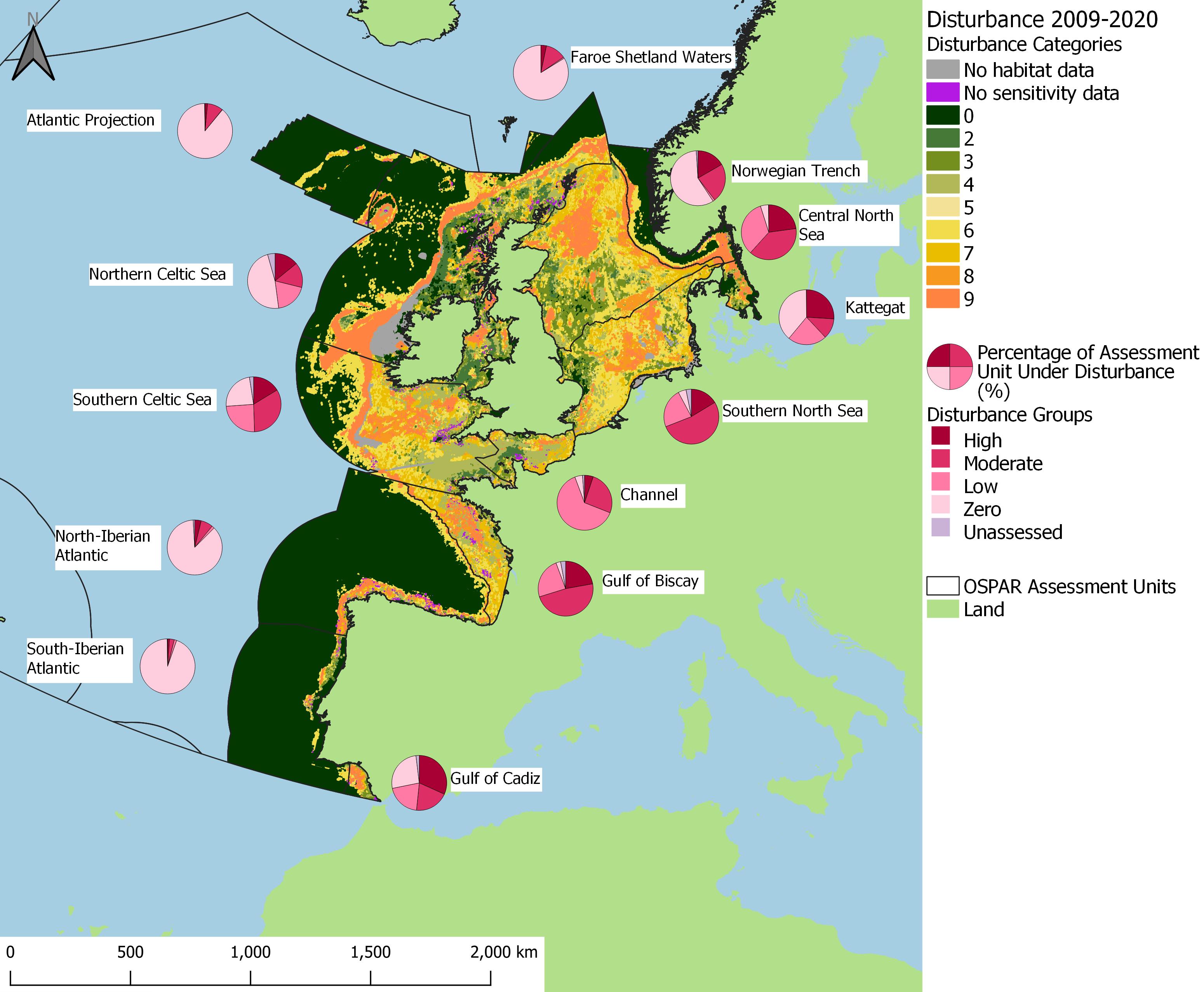
Figure 3: Spatial distribution of aggregated disturbance using the 2009 to 2020 assessment period. Pie chart plots show the percentage of the assessment unit area under each disturbance group: ‘Zero’ = disturbance category 0; ‘Low’ = disturbance categories 1 to 4; ‘Moderate’ = disturbance categories 5 to 7; ‘High’ = disturbance categories 8 and 9; ‘Unassessed Disturbance’ = area where fishing pressure was present, but disturbance could not be assessed due to i) no habitat data, or ii) no sensitivity assessments for underlying habitat
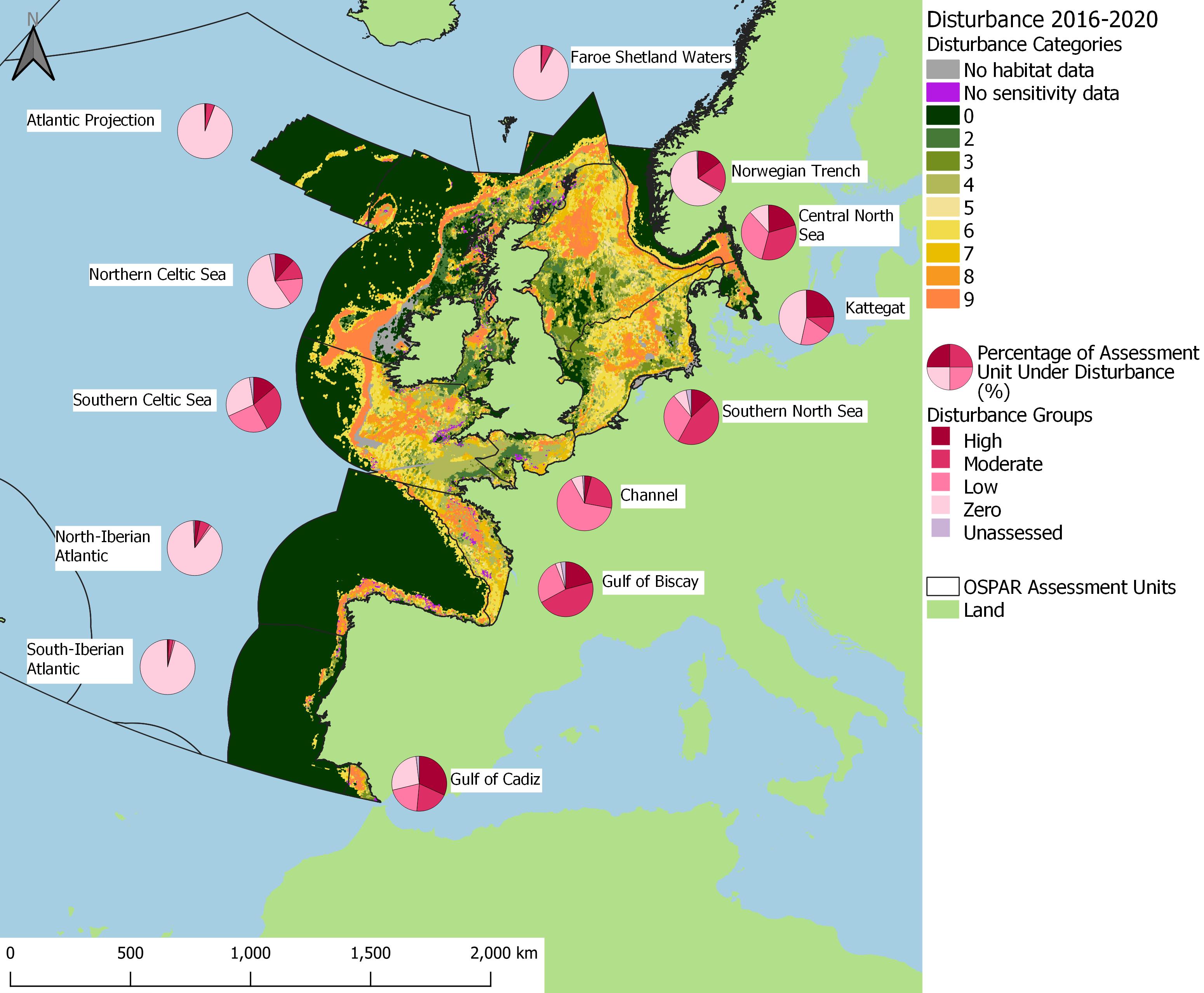
Figure 4: Spatial distribution of aggregated disturbance using the 2016 to 2020 assessment period. Pie chart plots show the percentage of the assessment unit area under each disturbance group: ‘Zero’ = disturbance category 0; ‘Low’ = disturbance categories 1-4; ‘Moderate’ = disturbance categories 5-7; ‘High’ = disturbance categories 8 and 9; ‘Unassessed Disturbance’ = area where fishing pressure was present, but disturbance could not be assessed due to i) no habitat data, or ii) no sensitivity assessments for underlying habitat
Total disturbance across all Common Indicator Assessment Units:
- Disturbance occurred in 53% (QSR) and 48% (MSFD) of the total assessed area as measured at the level of 0,05° x 0,05° c-squares.
- In the QSR assessment, 13% of the assessed area had ‘High’ disturbance, 23% ‘Moderate’, 18% ‘Low’, and 45% ‘Zero’ disturbance. In the MSFD assessment, 11% had ‘High’ disturbance, 19% ‘Moderate’, 18% ‘Low’, and 50% ‘Zero’ disturbance.
Percentage of assessment unit area in each disturbance group:
- The Gulf of Biscay had the greatest percentage of area with ‘High’ and ‘Moderate’ disturbance combined (QSR:70%; MSFD:67%), followed by the Southern North Sea (QSR:69%; MSFD:58%).
- The Gulf of Cadiz had the greatest percentage of area with ‘High’ disturbance (32%). The Channel had the highest percentage of area with ‘Low’ disturbance (QSR:63%; MSFD:64%).
- ‘Zero’ disturbance was greatest in the South-Iberian Atlantic (QSR: 94%; MSFD: 95%) and was most prevalent in assessment units with large areas of deep-sea habitat unsuitable for bottom-contact fishing.
- No clear disturbance trends were observed.
Habitat disturbance across all assessment units:
- All distinct BHTs had ‘High’ and / or ‘Moderate’ disturbance across all assessed area.
- BHTs with at least 50% of their area with ‘High’ or ‘Moderate’ disturbance (QSR and MSFD assessments): Upper bathyal sediment, Offshore circalittoral sand, and Offshore circalittoral mud; QSR assessment only: Infralittoral mixed sediment, Circalittoral mud and Circalittoral sand.
- ‘High’ disturbance was greatest in Offshore circalittoral mud (QSR:87%; MSFD:79%).
- ‘Low’ disturbance was greatest in Offshore circalittoral coarse sediment (QSR:91%; MSFD:87%).
- At a marine-assessment unit-scale, 75% of BHTs present within assessment units had ‘High’ and / or ‘Moderate’ disturbance in the QSR assessment; 70% in the MSFD period.
- All Circalittoral habitats present in assessment units had ‘High’ and / or ‘Moderate’ disturbance. Additionally, Circalittoral mixed sediment, Circalittoral mud, Offshore circalittoral mud, and Upper bathyal sediment all had ‘High’ disturbance.
- Offshore circalittoral mud had the greatest proportion of ‘High’ disturbance in most assessment units (QSR:9/11 units; MSFD:8/11 units).
- Offshore circalittoral sand had the greatest proportion of ‘Moderate’ disturbance in most assessment units (QSR:10/11 units; MSFD:8/11 units).
- The greatest proportions of ‘Low’ disturbance within assessment units were observed in two habitats: Offshore circalittoral coarse sediment (QSR:8/11 units; MSFD:7/11 units); and Offshore circalittoral mixed sediment (QSR:2/11 and MSFD:2/11 units).
- The greatest proportions of ‘Zero’ disturbance were observed in abyssal and lower bathyal BHTs, Upper bathyal and Offshore circalittoral rock and biogenic reef.
- ‘High’ disturbance in the Gulf of Cadiz was attributed to ‘High’ disturbance in Offshore circalittoral mud and Circalittoral mud.
- ‘Low’ disturbance in the Channel was attributed to ‘Low’ disturbance in Offshore circalittoral coarse sediment.
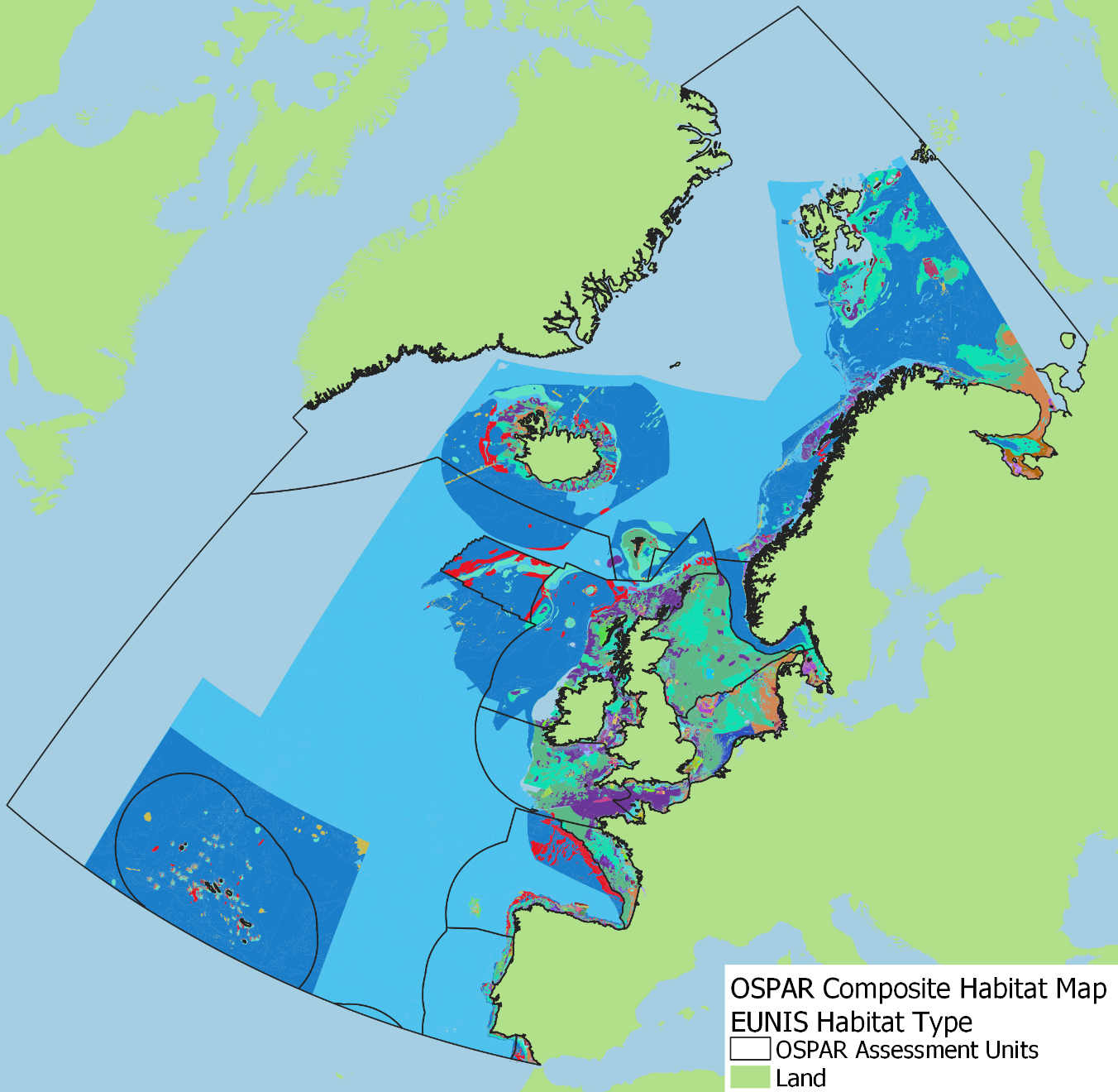
Figure a: OSPAR-scale composite habitat map symbolised at EUNIS Levels 2-6, integrating maps from surveys and broad-scale models
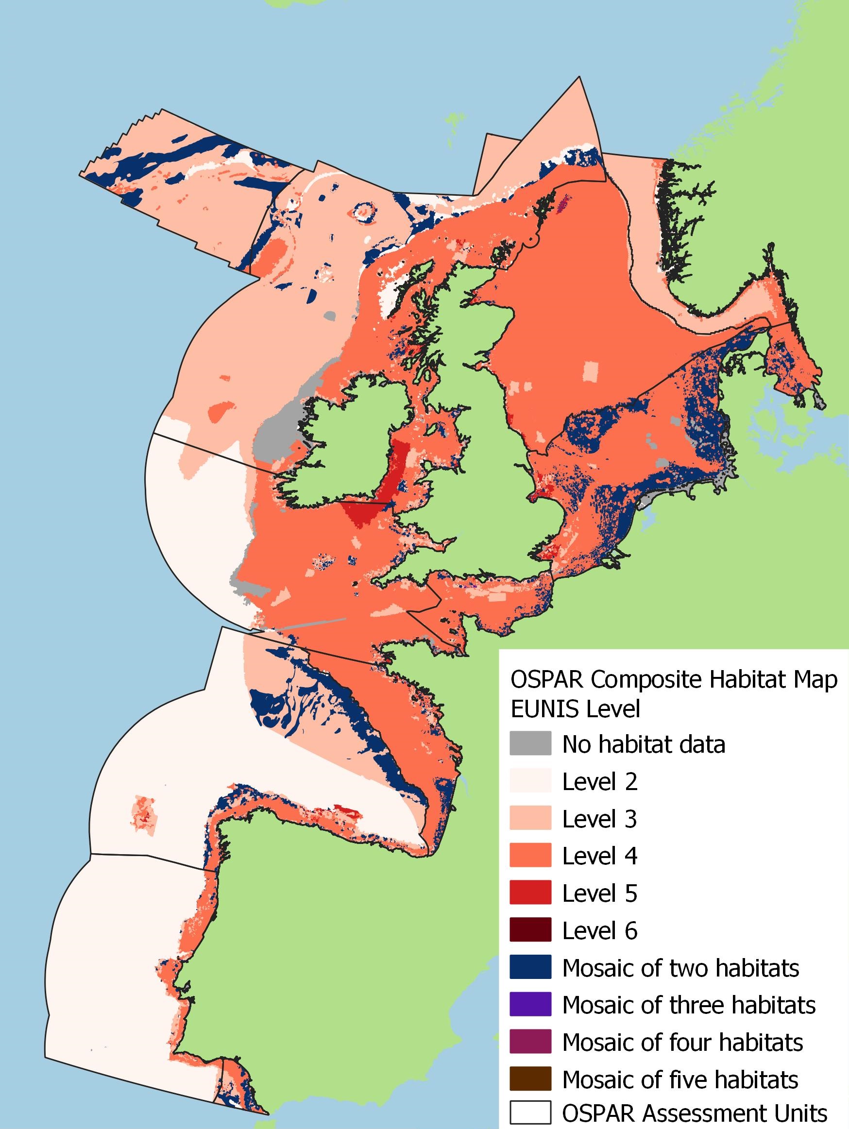
Figure b: OSPAR-scale composite habitat map, mapped at the most detailed EUNIS level for all assessment units considered under BH3. Where multiple EUNIS habitats are present, the number of habitats comprising the mosaic is given
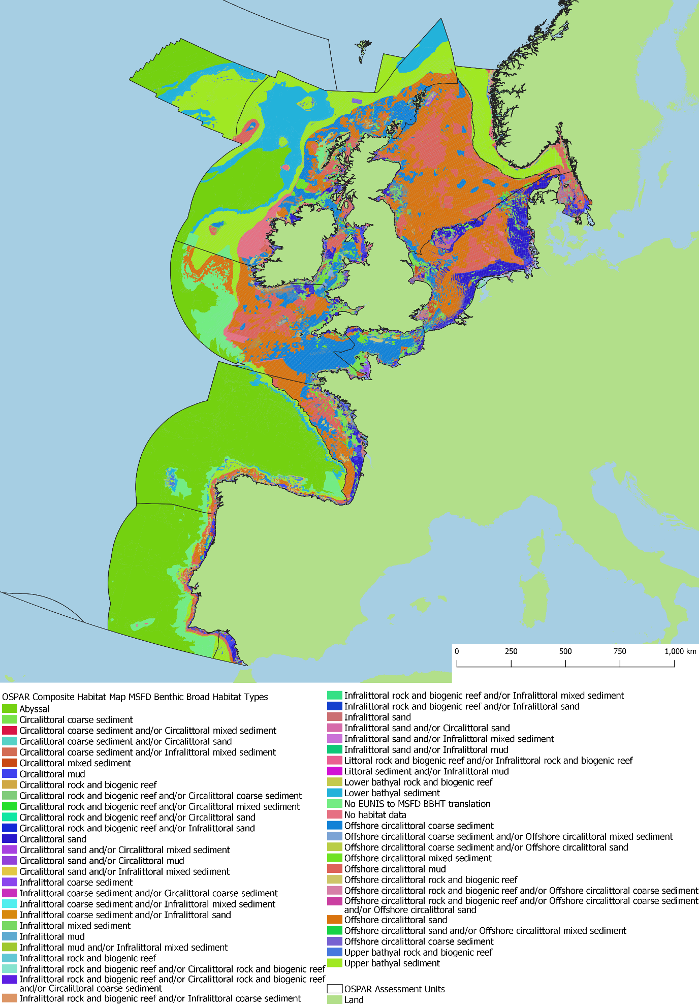
Figure c: OSPAR-scale composite habitat map in the MSFD Benthic Broad Habitat Type classification. Note that this map was created by translating EUNIS habitat codes within the OSPAR Composite Habitat Map to BHTs. Translations were conducted on the final disturbance outputs
In total, 362 distinct EUNIS 2007 codes and mosaic habitats were present in the composite habitat map. The composition of predominant broadscale EUNIS habitats between assessment units are summarised in Figure a and Figure d. Sublittoral coarse sediment (A5.1) habitats were the predominant habitats in the Channel and also represented a large proportion of the Southern Celtic Sea and Gulf of Biscay. Sublittoral sand (A5.2) habitats were predominant in the Central North Sea and Southern North Sea, although also represented a large proportion of habitat within the Kattegat, Southern Celtic Sea, and Gulf of Biscay assessment units. Sublittoral mud (A5.3) habitats represented the largest proportion of the Kattegat, although they were also present as a large proportion of the Central North Sea, Gulf of Biscay, and Gulf of Cadiz. Visualisations of analyses were presented for predominant EUNIS habitats; for the purpose of this assessment, predominant EUNIS habitats were defined as those with coverage greater than 1% of the total assessed area.
To facilitate reporting against Article 8 of the MSFD, EUNIS classified habitats were translated to BHT (Figure c), where EUNIS habitat data were available in the composite habitat map and direct translations were feasible. However, it should be noted that some areas of EUNIS habitat data were missing from the composite habitat map (e.g., the west coast of Ireland; south-west of Ireland; along the coast of the Netherlands, Germany, Denmark, and Norway; and the Ise Fjord, Roskilde Fjord and Øresund strait of the Kattegat assessment unit). Less than 5% of the area with available EUNIS habitat codes could not be translated to a BHT due to a lack of necessary habitat information (e.g., only EUNIS Level 2 data available without substrate information), predominantly in deep-sea (A6) areas. Additionally, certain habitats could only be translated to two or more potential BHTs. Data visualisations of analyses were presented for distinct BHT types only; inconclusive translations (e.g., multiple potential BHTs) accounted for < 0,1% (Figure e) of the total area of Common Indicator Assessment Units, and were not shown in graphs to maximise clarity and understanding for end users (Figure f). Data gaps in the composite habitat map resulted from constraints associated with the input data used to create the map product, such as limited spatial extent of EUSeaMap (EMODnet, 2021). The underlying habitat layer presented in Figure a and Figure c was used for both the 2009 to 2020 and 2016 to 2020 disturbance assessments.
The composition of assigned BHTs varied between assessment units (Figure f). Some assessment units showed similar proportions of predominant habitats; both Northern-Iberian Atlantic and Southern-Iberian Atlantic were predominantly Abyssal in biological zone and depth; Faroe Shetland Waters, Norwegian Trench, Northern Celtic Sea, and Gulf of Cadiz were predominantly classified as Upper bathyal sediment, whereas the Central North Sea, Southern North Sea, Southern Celtic Sea, and Gulf of Biscay were predominantly Offshore circalittoral sand or Circalittoral sand. The Channel was predominantly Offshore circalittoral coarse sediment and the Kattegat was predominantly Offshore circalittoral mud and infralittoral sand.
Figure d: Aggregated EUNIS level 2, level 3, and mosaic habitats with at least 1% coverage in any assessment unit. No EUNIS data = area of assessment unit where EUNIS habitat data were not available (habitat information unavailable or incompatible with EUNIS classification)
Figure e: The percentage of the total OSPAR common indicator area that each BHT covered. Additionally, the percentage of the total assessed area where there was no EUNIS data and where no EUNIS to BHT translation was possible is also represented
Figure f: Proportion of BHT following translation from EUNIS; inconclusive translations (e.g., multiple potential BHTs) not shown (<0.1% total area). No EUNIS to BHT translation = EUNIS habitats that couldn’t be assigned MSFD translations (e.g., lacking substrate information); No EUNIS data = area of assessment unit where EUNIS habitat data were not available (habitat information unavailable or incompatible with EUNIS classification). The blue shading distinguishes between habitats of different biological zones, the red shading distinguishes No EUNIS data / No EUNIS to BHT translation from BHTs
Sensitivity
The use of aggregated MarESA sensitivity scores enabled fine-scale biotope-resolution sensitivity to be mapped at all EUNIS Levels, demonstrating a clear improvement in accuracy of assessments from the IA 2017. However, it should be noted that increased coverage of habitat sensitivity information (from aggregations) resulted in sensitivity being available for broadscale EUNIS habitats (e.g., EUNIS Level 2). Habitats at Level 2 of the EUNIS classification or where direct translations between EUNIS 2007 and MSFD BHTs were not possible required additional information, such as substrate type, to enable translation to MSFD BHT. Where additional habitat information required for translation was not available from EUSeaMap 2021, results were not summarised to a BHT. Less than 5% of the area with assessment results could not be translated to a BHT; more sensitivity information was available in the EUNIS classification than could be translated to BHT.
Assessment units with large areas of deep-sea predominantly had sensitivity categories 4 and 5 (Figure g and Figure h). Faroe Shetland Waters, the Norwegian Trench, North-Iberian Atlantic, and South Iberian Atlantic had the highest proportions of surface sensitivity category 5 (99%, 71%, 93%, and 91% respectively; Figure i). Deep-sea habitats and their component species (e.g., cold-water corals) typically experience slow rates of change in environmental conditions, and taxa can form over long periods of time (Last et al., 2019a; Last et al., 2019b; Garrard et al., 2019; Garrard et al., 2020). Slow growth rates, combined with low reproduction rates can result in low resistance and resilience and therefore, high sensitivity to pressure.
Large areas of the continental shelf with sensitivity category 4 were typically associated with Sublittoral mud (A5.3; Figure a, Figure g and Figure h). Habitat sensitivity to surface and subsurface abrasion was broadly similar, with exceptions, such as habitats where subsurface abrasion pressure was not considered relevant (e.g., some circalittoral rock biotopes) or where habitats were less sensitive to surface abrasion (e.g., sublittoral sand). Assessment units with large ratios of sand or coarse sediment habitats (Central North Sea, Southern North Sea, Southern Celtic Sea, Gulf of Biscay, and Channel) correspondingly had large proportions of habitat area with sensitivity values of 2 or 3 (Figure i). Conversely, Abyssal and bathyal BHTs were all consistently categorised with high sensitivities (Figure j and Figure k). The Norwegian Trench assessment unit had the largest proportion of unassessed sensitivity area; this was mostly attributed to the prevalence of unassessed biotopes such as A4.33 (Faunal communities on deep low energy circalittoral rock) and a lack of habitat information in coastal areas.
Figure g: Extent and distribution of habitat and benthic species sensitivities (based on resilience and resistance) to surface abrasion combined within EUNIS Level 2-6 benthic habitat types
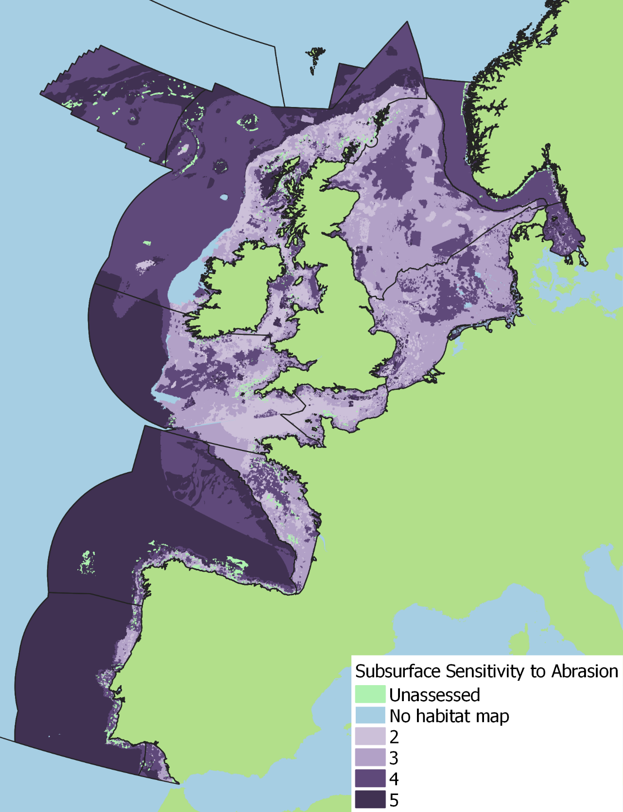
Figure h: Extent and distribution of habitat and benthic species sensitivities (based on resilience and resistance) to subsurface abrasion combined within EUNIS Level 2-6 benthic habitat types
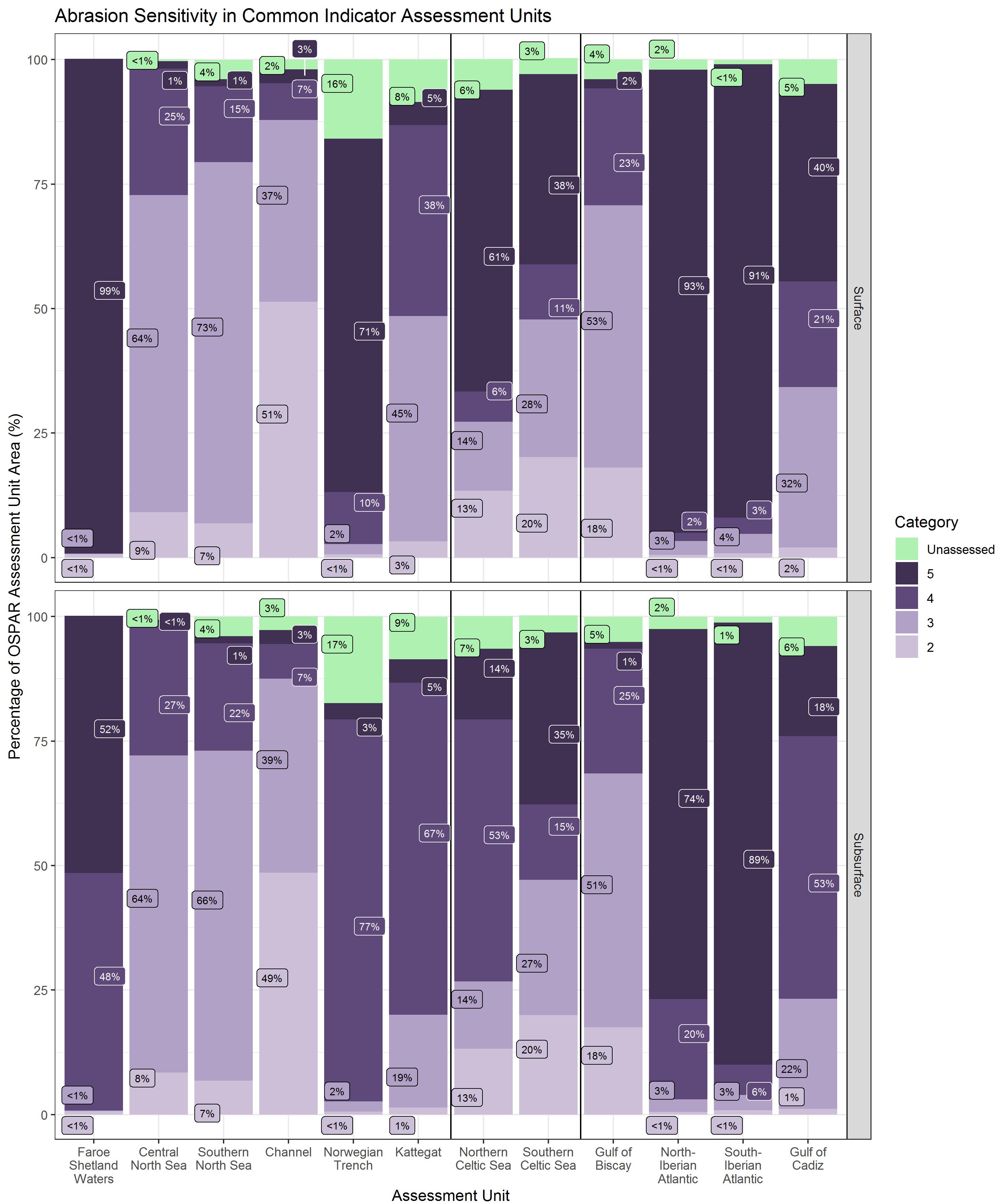
Figure i: Proportion of habitat and benthic species sensitivities (based on resilience and resistance) to surface and subsurface abrasion
Habitats that were unable to be translated from EUNIS to BHT (due to insufficient habitat resolution of detail) were predominantly recorded as having high sensitivity, as these were broadscale (e.g., EUNIS Level 2) and, therefore, likely had highly sensitive child biotopes resulting in high sensitivity following precautionary aggregations. The largest proportion of area with unassessed sensitivity was observed in Rock and biogenic reef BHTs which typically related to EUNIS rock habitats (e.g., ‘Faunal communities on deep moderate energy circalittoral rock A4.27 EUNIS 2007’). Unassessed sensitivity in Rock and biogenic reef BHTs typically related to ‘rock’ habitats unlikely to be targeted by bottom-contacting fishing, and therefore assessments of surface or subsurface abrasion from fishing gear were not relevant or not assessed.
Where rock and biogenic habitats had sensitivity assessments, they were mostly sensitivity categories 4 or 5. Offshore circalittoral mud was almost entirely assessed as surface sensitivity category 4 across all assessment units, whereas circalittoral and infralittoral mud surface sensitivity categories varied across assessment units (Figure j). However, circalittoral and infralittoral mud was predominantly sensitivity category 4 across all assessment units for subsurface abrasion. The sensitivity categories of mixed sediment BHTs varied across assessment units but were frequently categorised as more sensitive in the infralittoral and circalittoral biological zone than in offshore areas (Figure k).
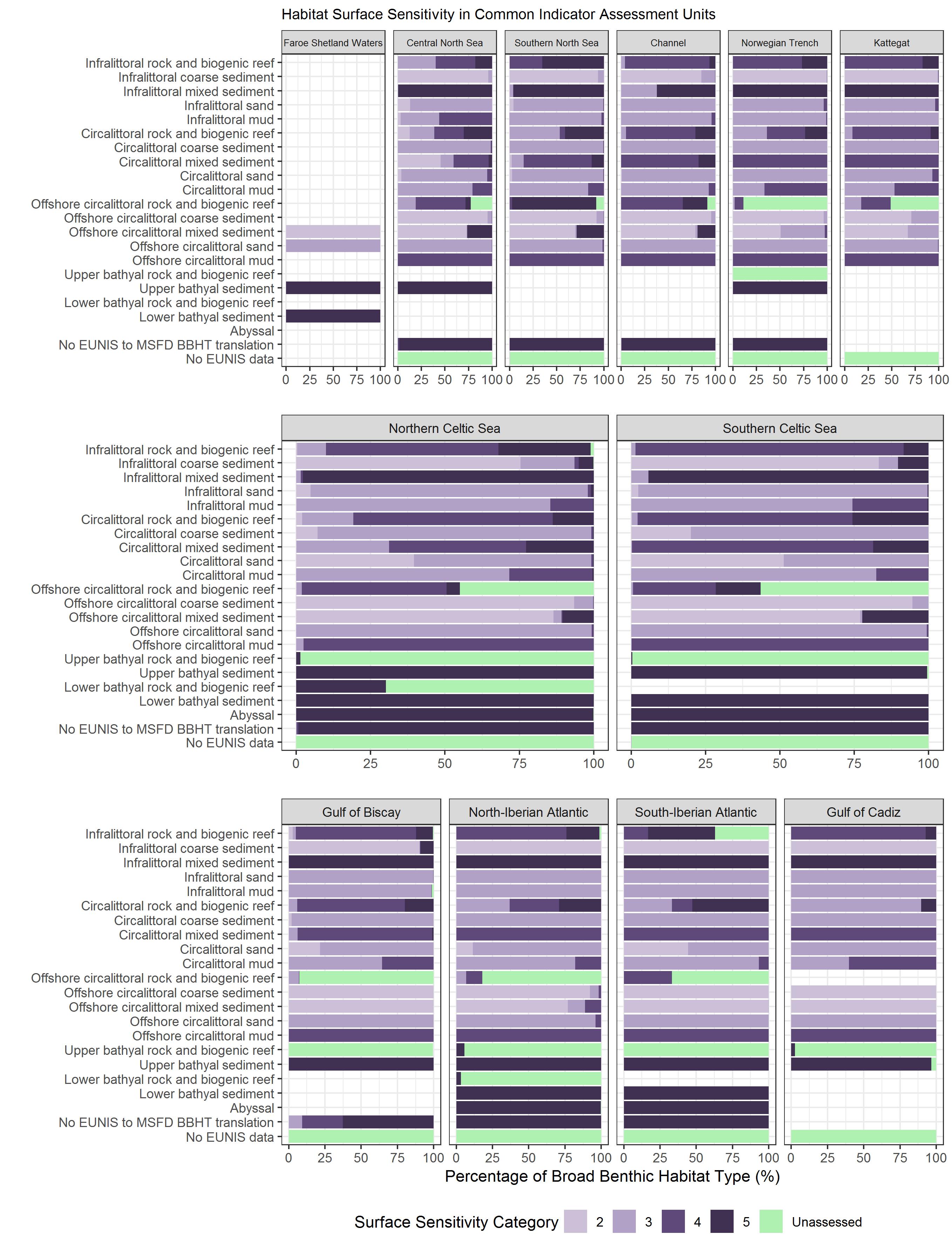
Figure j: Proportion of surface sensitivity categories for BHTs following translation from EUNIS; inconclusive translations (e.g., multiple potential BHTs) not shown (<0.1% total area). No EUNIS to BHT translation = EUNIS habitats that couldn’t be assigned MSFD translations (e.g., lacking substrate information); No EUNIS data = area of assessment unit where EUNIS habitat data were not available (habitat information unavailable or incompatible with EUNIS classification)
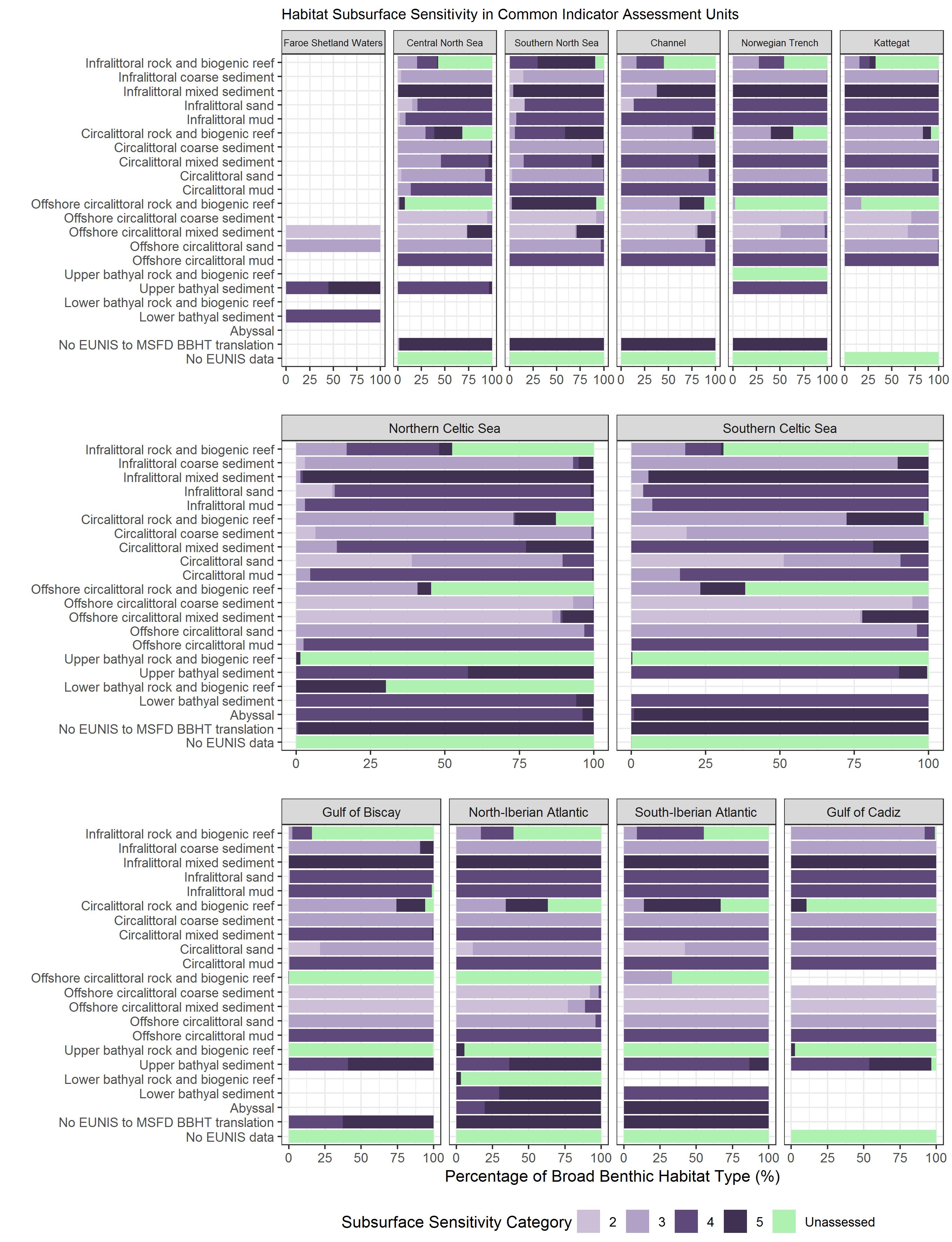
Figure k: Proportion of subsurface sensitivity categories for BHTs following translation from EUNIS; inconclusive translations (e.g., multiple potential BHTs) not shown (<0.1% total area). No EUNIS to BHT translation = EUNIS habitats that couldn’t be assigned MSFD translations (e.g., lacking substrate information); No EUNIS data = area of assessment unit where EUNIS habitat data were not available (habitat information unavailable or incompatible with EUNIS classification)
Pressure
2009 to 2020:
The extent of surface abrasion categories of 4 and 5 were widespread in shallow and shelf areas (Figure l). The assessment unit with the highest percentages of pressure category 5 was the Gulf of Biscay (59%), closely followed by the Channel (47%), the Southern Celtic Sea (32%), Central and Southern North Sea (32% and 22%, respectively), and the Gulf of Cadiz (28%) (Figure o).
Shelf areas of assessment units that had lower levels of pressure (1) included southern parts of the Central North Sea; central areas of the Channel; some areas of the Irish Sea; and offshore areas of the west coasts of Scotland and Ireland (Figure l). Low surface abrasion categories (1 and 2) were found in deep-sea areas such as the Norwegian Trench and Biscay Abyssal Plain. The lack of pressure in the coastal areas of the Southern-Iberian Atlantic possibly occurred due to unreported VMS fleet data.
Variability in surface fishing pressure in the assessment period 2009 to 2020 (Figure n) was widespread across most assessment units with the Central North Sea having the largest proportion of area categorised as ‘Variable’ (44%), followed by the Southern North Sea (42%) (Figure o). Assessment units that showed the highest percentages of ‘Consistent’ fishing were the Channel (77%) and Gulf of Biscay (71%), followed closely by Southern Celtic Sea (55%), Kattegat (55%), and Southern and Central North Sea (53% and 51% respectively). Furthermore, a large variation was observed in surface abrasion categories and the area in which pressure occurred in the Gulf of Cadiz (29%).
In areas of ‘Consistent’ fishing, those with the highest surface abrasion pressure categories (4 or 5) were found in the Skagerrak area, central and southern areas of the Southern North Sea, the Channel, Irish Sea, Southern Celtic Sea, and Gulf of Biscay (Figure p). In most assessment units, the majority of Offshore circalittoral mud had the highest or second highest-pressure categories (4 or 5) (Figure q). Offshore circalittoral BHTs typically had the greatest proportion of area with surface abrasion pressure, many with more than 75% of the total habitat area with the highest-pressure categories (4 or 5).
The proportion of surface abrasion pressure in areas without EUNIS habitat information (due to a lack of habitat map coverage) was highest in Southern Celtic Sea, although only 3% of the Southern Celtic Sea lacked EUNIS information (Figure d and Figure q). EUNIS habitat data was lacking in only 4% of the area of the Southern North Sea, although, a high proportion of pressure categories 4 or 5 were present where EUNIS habitat data was missing (Figure d and Figure q). Widespread occurrences of surface abrasion pressure in areas without EUNIS habitat data in the Northern Celtic Sea was mostly attributed to the lack of habitat data off the west coast of Ireland.
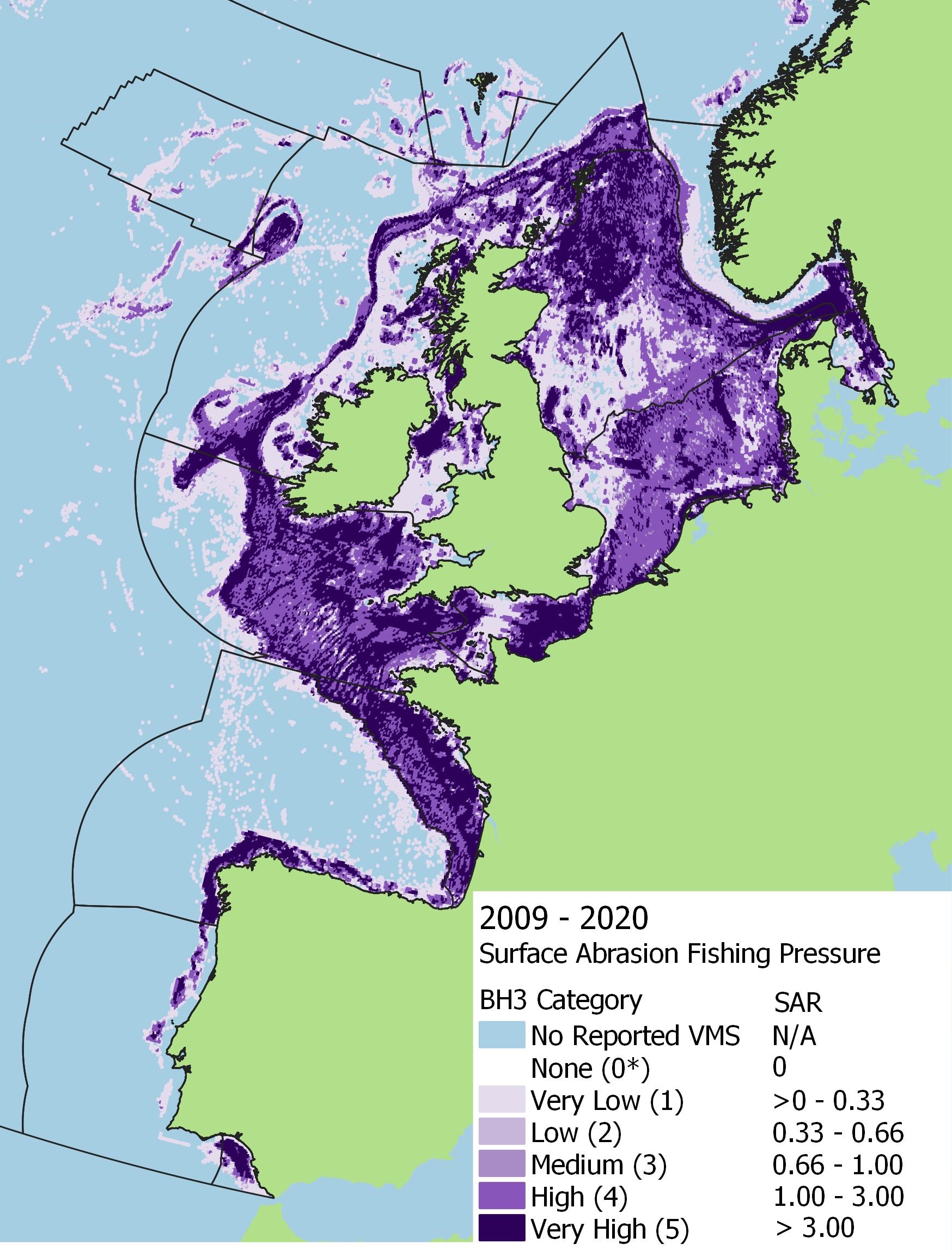
Figure l: Aggregate surface abrasion pressure in the 2009 to 2020 assessment period. Note, BH3 category 0* = 0 SAR value reported by ICES for vessels >12 m only
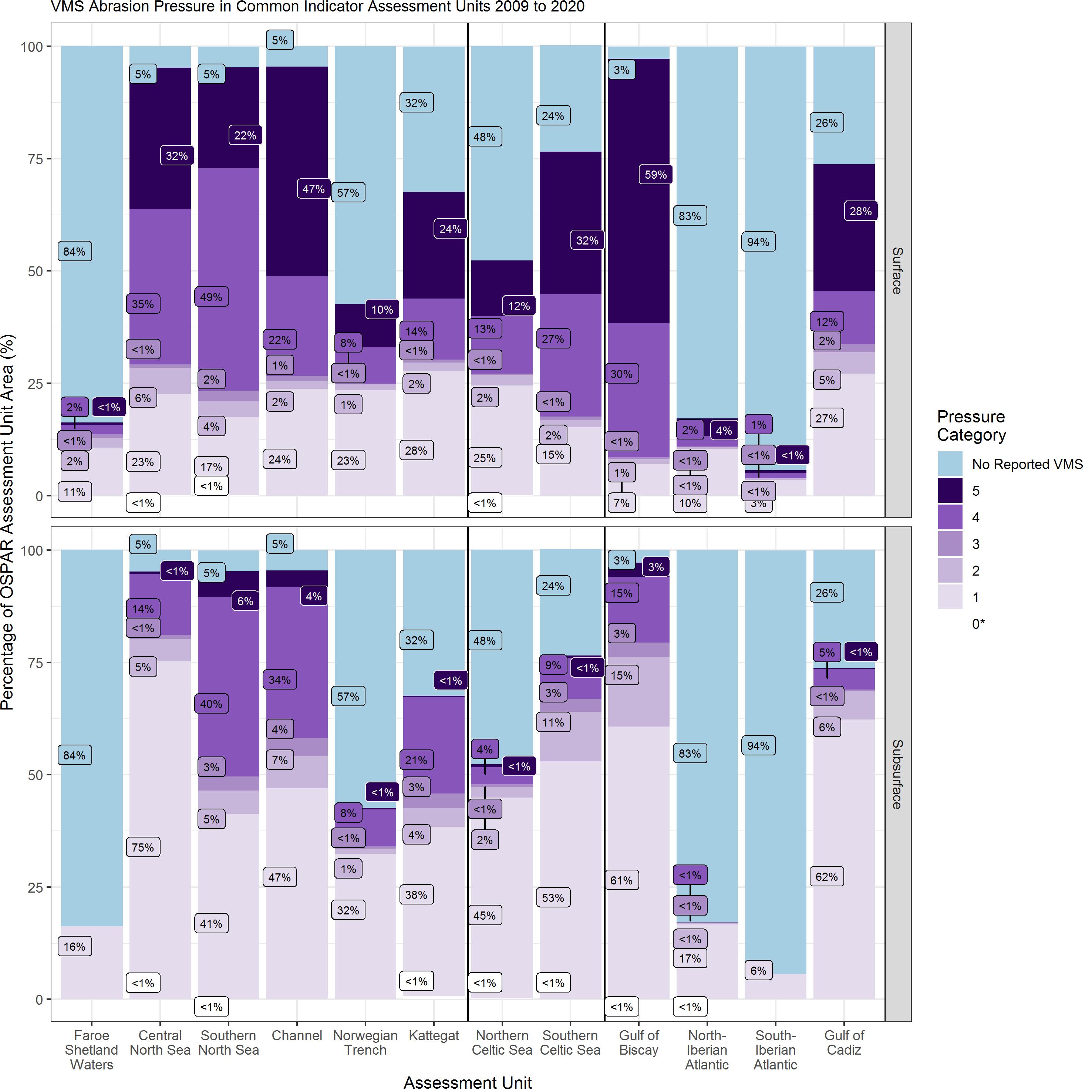
Figure m: Proportion of aggregated surface and subsurface abrasion pressure categories in the assessment period 2009 to 2020. Note, BH3 category 0* = 0 SAR value reported by ICES for vessels >12 m only
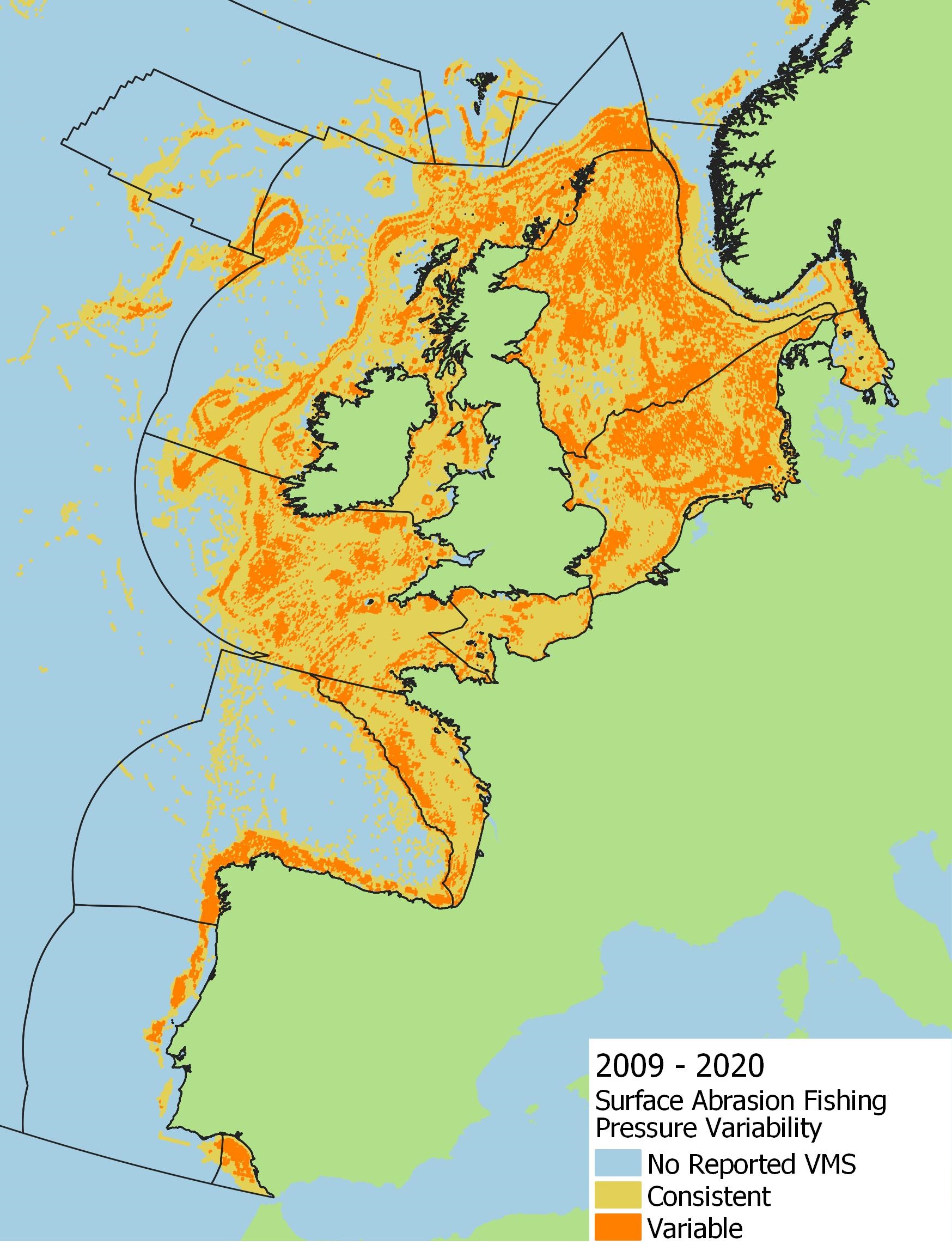
Figure n: Spatial distribution of ‘Variable’ and ‘Consistent’ surface fishing pressure in the 2009 to 2020 assessment period. C-squares were categorised ‘Variable’ if a range of three or more SAR categories was observed throughout the time series
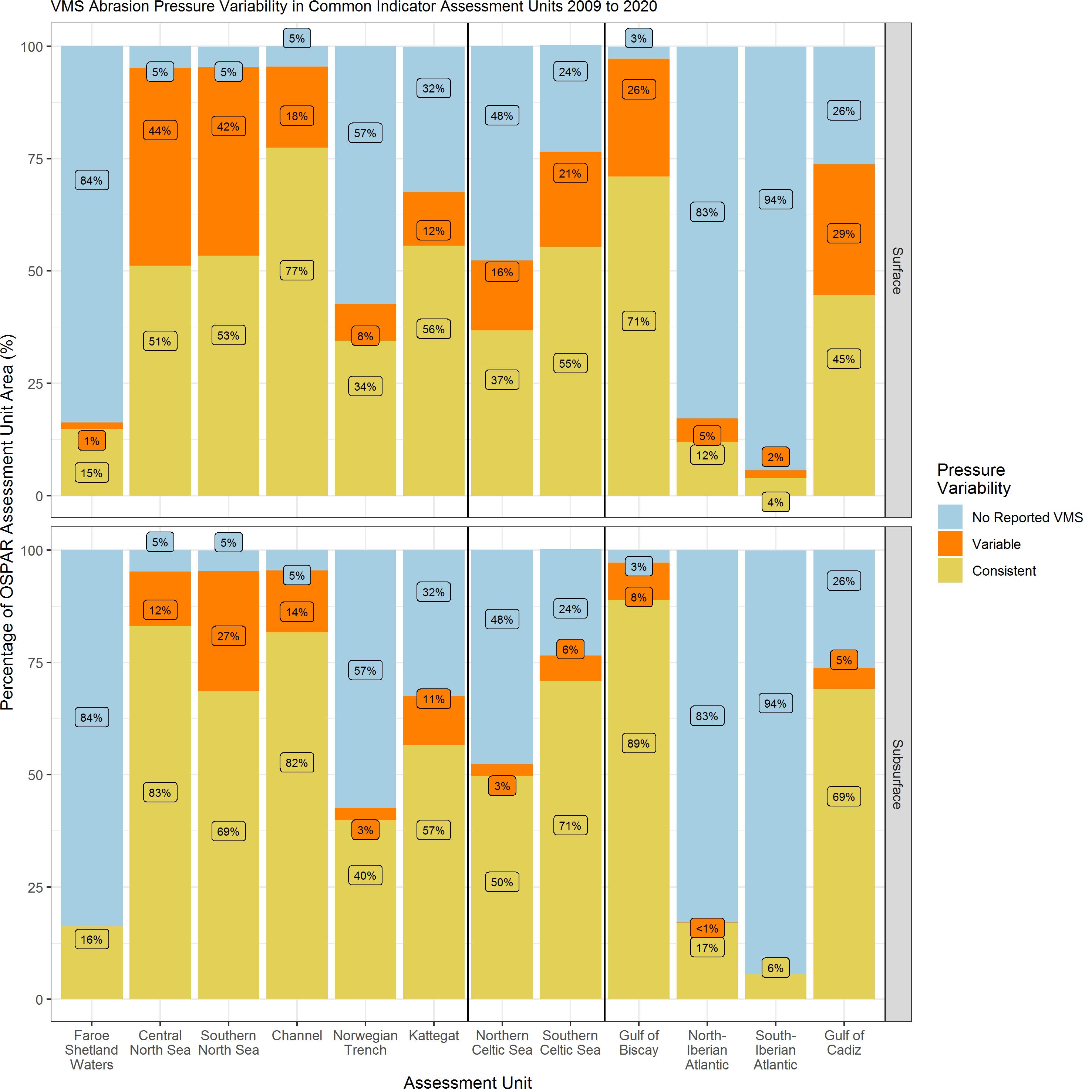
Figure o: Proportion of ‘Variable’, ‘Consistent’, and no VMS data in the assessment period 2009 to 2020. C-squares were categorised ‘Variable’ if a range of three or more SAR categories was observed throughout the time series
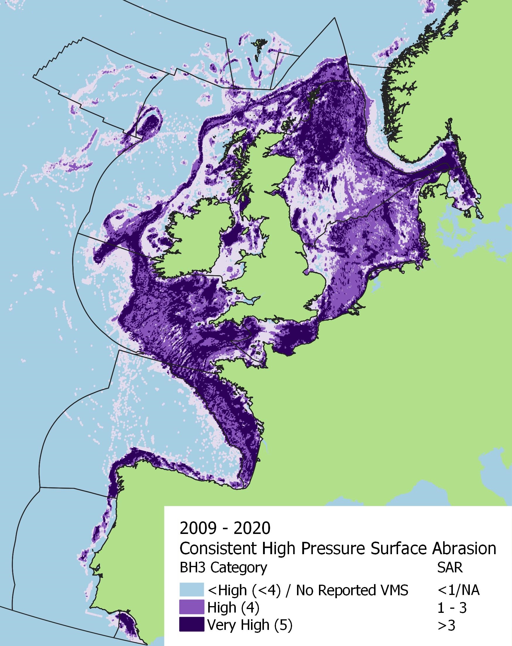
Figure p: Spatial distribution of consistently high (category 4 or 5) surface fishing pressure within the 2009 to 2020 assessment period. C-squares were considered to have ‘Consistent’ pressure if a change in less than three SAR categories was observed within the assessment period
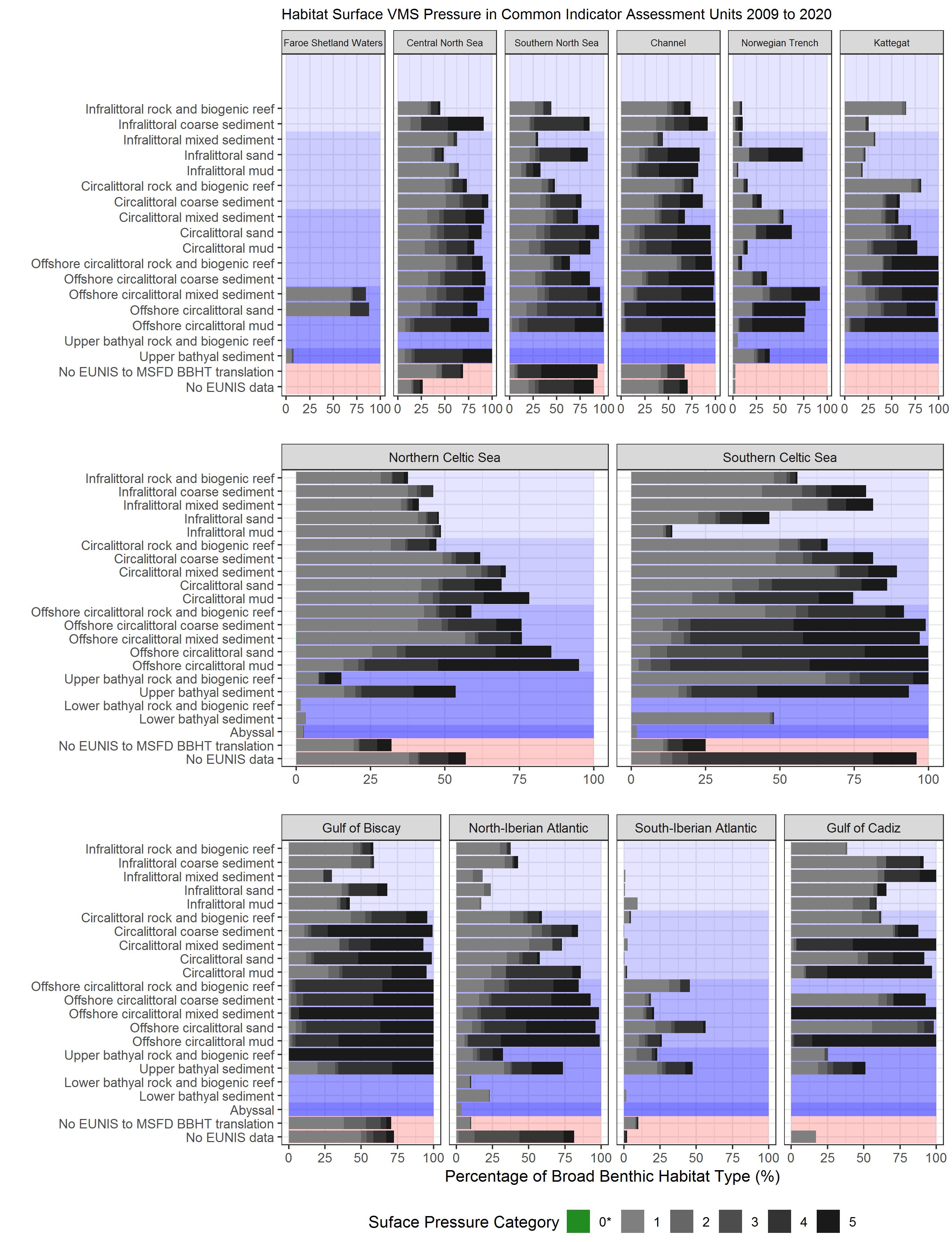
Figure q: Proportion of surface abrasion pressure categories in BHTs (excluding inconclusive translations) in the assessment period 2009 to 2020. 0* = 0 SAR value reported by ICES for vessels >12 m only. No EUNIS to BHT translation = EUNIS habitats that couldn’t be assigned MSFD translations (e.g., lacking substrate information); No EUNIS data = area of assessment unit where EUNIS habitat data were not available (habitat information unavailable or incompatible with EUNIS classification). The blue shading distinguishes between habitats of different biological zones, the red shading distinguishes No EUNIS data/No EUNIS to BHT translation from BHTs. Note, BH3 category 0* = 0 SAR value reported by ICES for vessels >12 m only
The highest aggregated subsurface abrasion categories were observed in the Southern North Sea, noticeable in the centre and along the Dutch, German and Belgian coastlines (6% in category 5, and 40% in category 4) (Figure m and Figure r). Higher aggregated subsurface abrasion categories (4 or 5) were observed in the eastern and western areas of the Channel the Skagerrak / Kattegat areas; the central Irish Sea area; Southern Celtic Sea; the west coast of Scotland; Porcupine Bank; and south of Brittany to the Medoc region in France (Gulf of Biscay). There was also a large extent of pressure category 4 observed in the Fladen Grounds area of the Central North Sea (Figure r).
Variability in subsurface fishing pressure in the assessment period 2009 to 2020 (Figure s) was greatest in the Southern North Sea (27%), followed by the Channel (14%), Central North Sea (12%; mainly around Fladen Grounds), and the Kattegat (11%) (Figure o). The assessment unit with the highest ‘Consistent’ subsurface abrasion was Gulf of Biscay (89%). Many areas with the highest subsurface abrasion categories (4 or 5) were also categorised as ‘Consistent’ pressure across the assessment period, which was most evident in the south of the Southern North Sea, the Kattegat and Skagerrak areas, the Channel, the central Irish Sea area, the Southern Celtic Sea, and the Gulf of Biscay (Figure t). The proportion of ‘Variable’ subsurface pressure was very low in the North Iberian-Atlantic and zero in the South-Iberian Atlantic.
In the assessment period 2009 to 2020, almost all (>98%) of Offshore circalittoral mud experienced subsurface pressure (with exceptions in the Norwegian Trench and South-Iberian Atlantic). Furthermore, Offshore circalittoral mud had more than 50% of area with the highest two subsurface pressure categories in the Kattegat, Southern North Sea, the Channel, and Norwegian Trench assessment units (Figure u). Offshore circalittoral mixed sediment experienced a high percentage of high subsurface pressure (4 and 5) in the Gulf of Biscay (65%). Offshore circalittoral sand experienced a high percentage of high subsurface pressure (4 and 5) in the Channel (84%) (Figure u). In contrast, the North and South-Iberian Atlantic assessments units displayed lower percentages of habitat areas with the highest categories of subsurface abrasion.
The proportion of subsurface abrasion pressure in areas without habitat information was broadly similar to that for surface pressure (Figure u). However, the proportion of area in which subsurface abrasion pressure categories 4 or 5 occurred was lower than equivalent categories for surface abrasion in all assessment units. Furthermore, the Southern North Sea showed a high proportion of area without EUNIS habitat data with subsurface pressure categories 4 or 5.
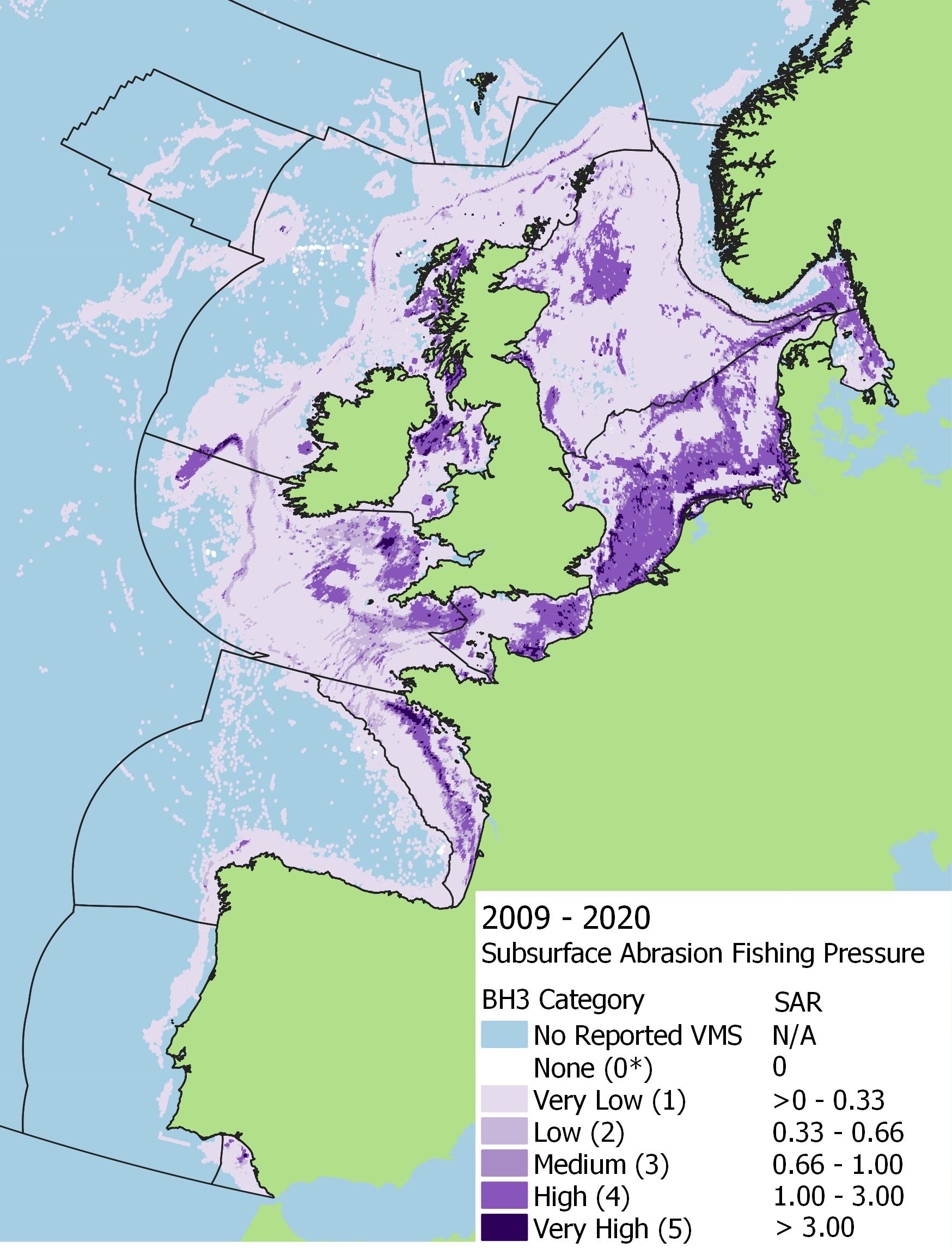
Figure r: Aggregated subsurface abrasion pressure in the 2009 to 2020 assessment period. Note, BH3 category 0* = 0 SAR value reported by ICES for vessels >12 m only
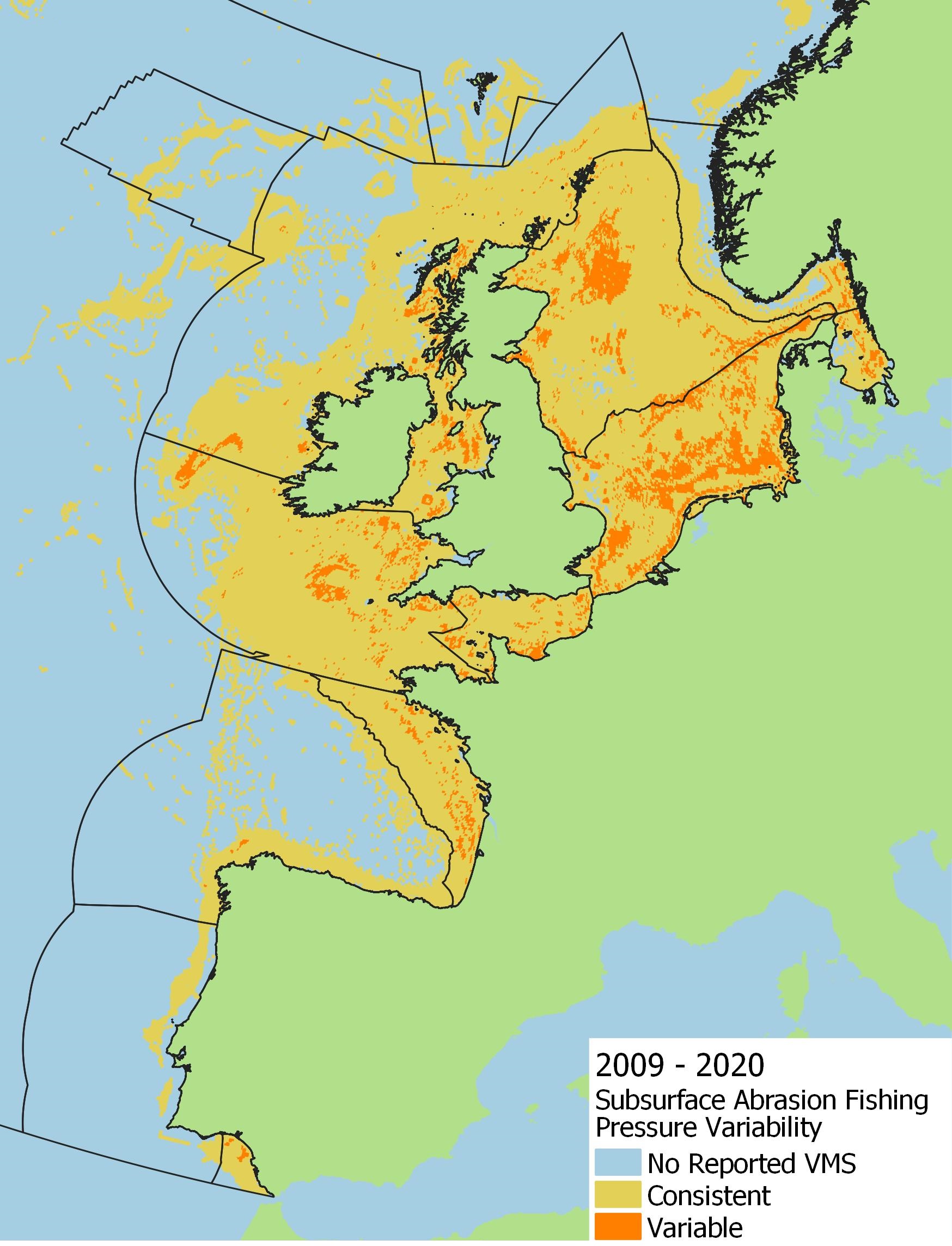
Figure s: Spatial distribution of ‘Variable’ and ‘Consistent’ sub-surface fishing pressure using the 2009 to 2020 assessment period. C-squares were categorised ‘Variable’ if a range of three or more SAR categories was observed throughout the time series
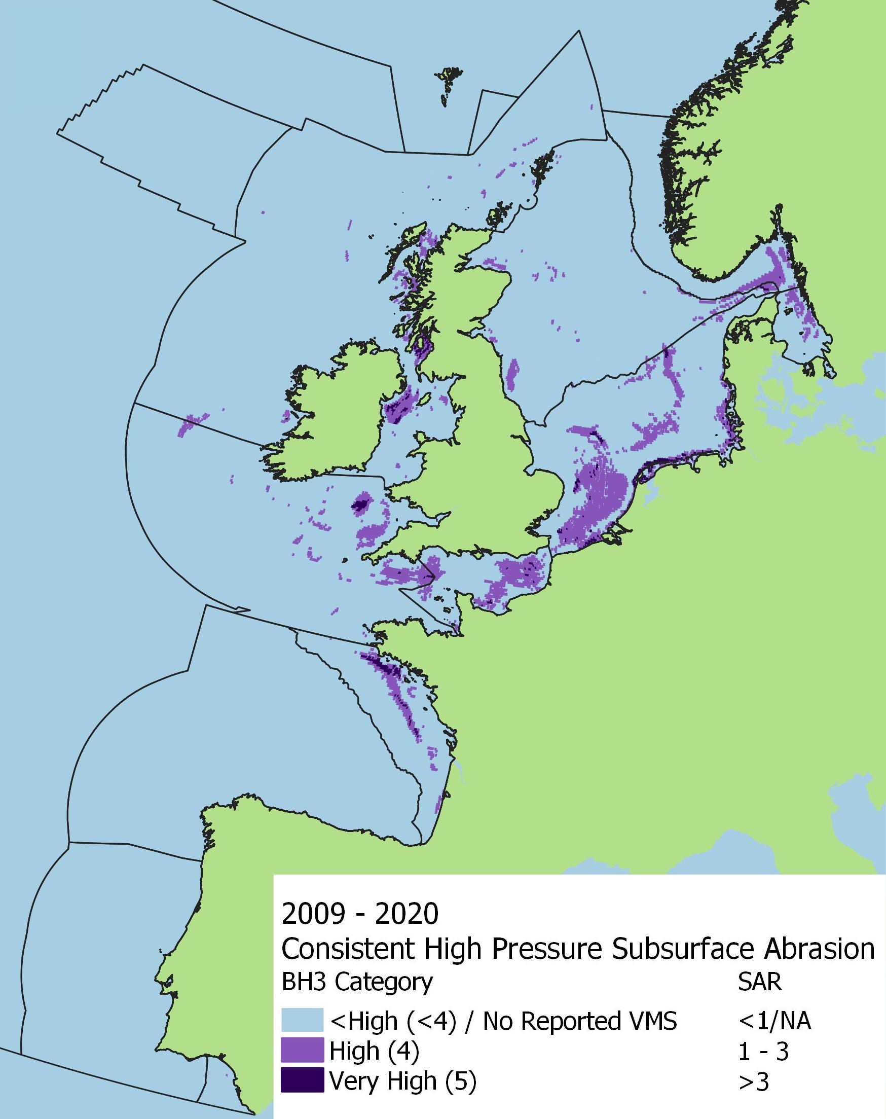
Figure t: Spatial distribution of consistently high (category 4 or 5) subsurface fishing pressure within the 2009 to 2020 assessment period. C-squares were considered to have ‘Consistent’ pressure if a change in less than three SAR categories was observed within the assessment period
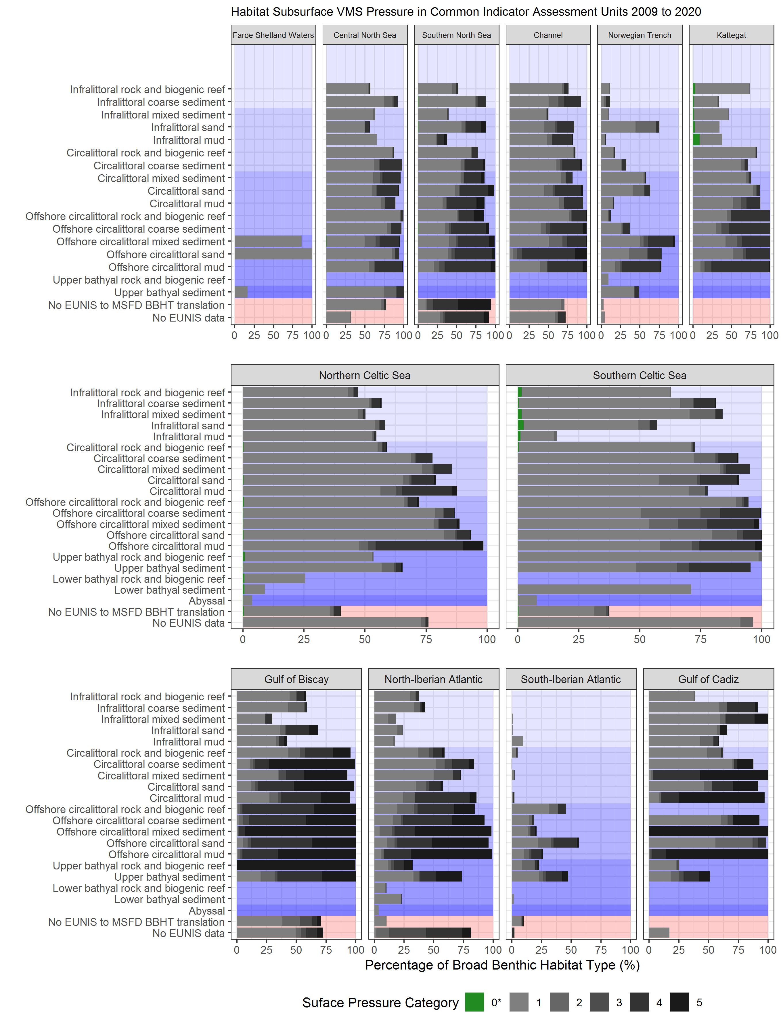
Figure u: Proportion of subsurface abrasion pressure categories in BHTs (excluding inconclusive translations) in the assessment period 2009 to 2020. 0* = 0 SAR value reported by ICES for vessels >12 m only. No EUNIS to BHT translation = EUNIS habitats that couldn’t be assigned MSFD translations (e.g., lacking substrate information); No EUNIS data = area of assessment unit where EUNIS habitat data were not available (habitat information unavailable or incompatible with EUNIS classification). The blue shading distinguishes between habitats of different biological zones, the red shading distinguishes No EUNIS data / No EUNIS to BHT translation from BHTs. Note, BH3 category 0* = 0 SAR value reported by ICES for vessels >12 m only
2016 to 2020:
Aggregated surface abrasion categories in the assessment period 2016 to 2020 are shown in Figure v. The extent of surface abrasion categories of 4 and 5 was widespread across the continental shelf and similar in distribution to those mapped in the assessment period 2009 to 2020, although there appeared to be a slight reduction in the distribution of areas of the highest values. Additionally, in the 2016 to 2020 assessment period, the highest surface abrasion was observed in the Gulf of Biscay (46% category 5), followed by the Channel (38% category 5) (Figure w).
Variability in surface fishing pressure in the assessment period 2016 to 2020 was widespread across most assessment units (Figure x), with the Central North Sea, Southern North Sea, and Gulf of Cadiz, having the largest proportions of area categorised as ‘Variable’ (~16-17%) (Figure y). Similar to the 2009 to 2020 assessment period many areas with the highest surface abrasion categories were also categorised as ‘Consistent’ (Figure z; south of the Southern North Sea, the Kattegat and Skagerrak areas, the Channel, the central Irish Sea area, the Southern Celtic Sea, and the Gulf of Biscay). The assessment units with the highest ‘Consistent’ values of surface abrasion were the Channel (89%) and Gulf of Biscay (88%), followed closely by Southern North Sea and Central North Sea. Direct comparison of the total area categorised as ‘Consistent’ or ‘Variable’ pressure was not considered possible between the two assessment periods as the QSR interval included the data in the MSFD assessment period, and additional variations in legislative VMS data reporting requirements.
Habitats with large proportions of area with surface pressure categories 0-5 in the assessment period 2016 to 2020 are summarised in Figure aa. As observed in the 2009 to 2020 period, in almost all regions, Offshore circalittoral mud habitat had the majority of area with the two highest pressure categories. In most assessment units, there were multiple habitats with large proportions of area in the highest surface pressure categories (4 or 5), most noticeable in the Southern North Sea, Channel and Gulf of Biscay.
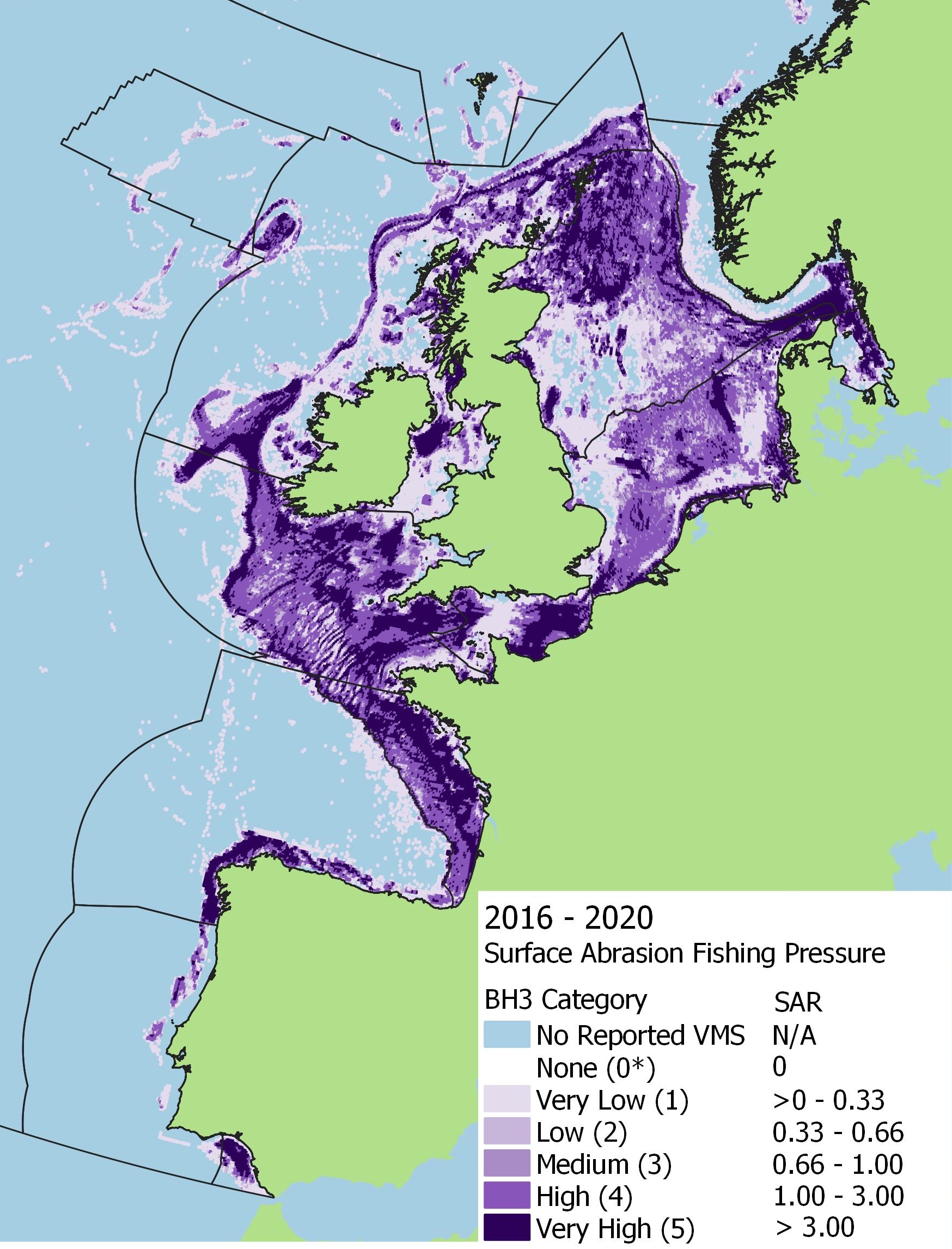
Figure v: Aggregated surface abrasion pressure in the 2016 to 2020 assessment period. Note, BH3 category 0* = 0 SAR value reported by ICES for vessels >12 m only
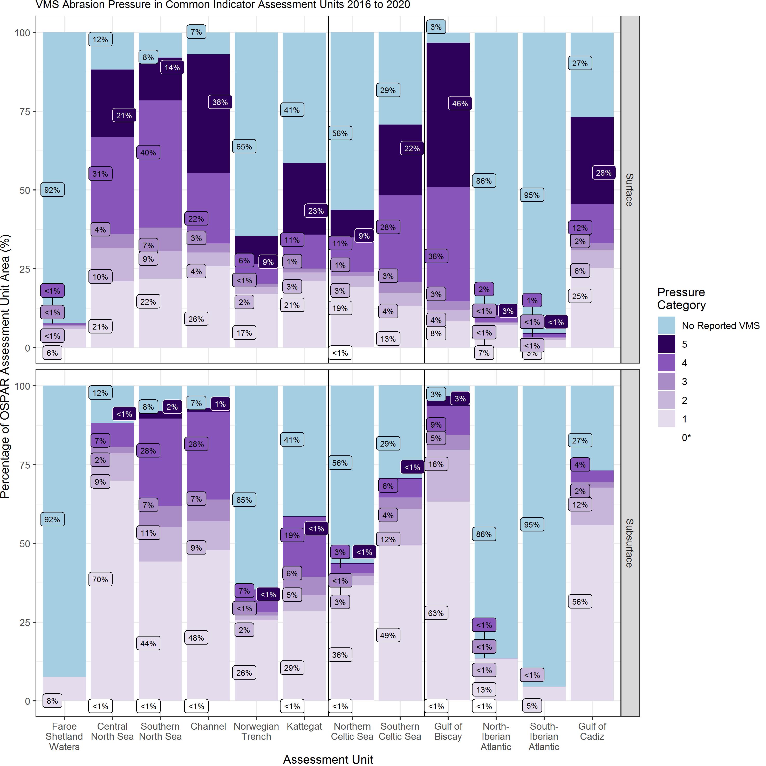
Figure w: Proportion of aggregated surface and subsurface abrasion pressure categories in the assessment period 2016 to 2020. Note, BH3 category 0* = 0 SAR value reported by ICES for vessels >12 m only
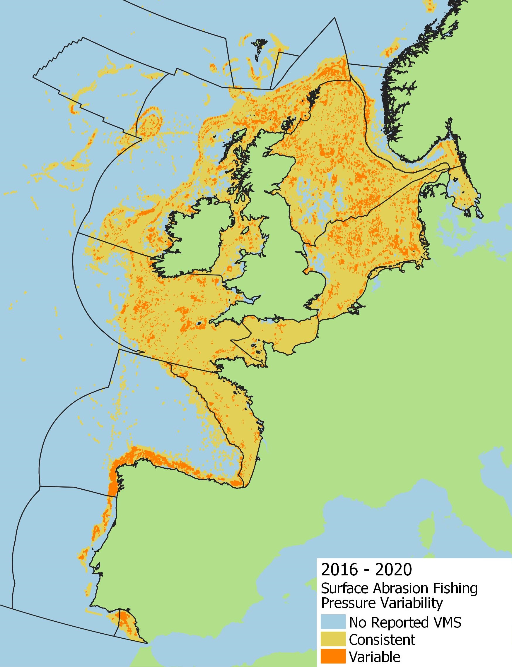
Figure x: Spatial distribution of ‘Variable and ‘Consistent’ surface fishing pressure using the 2016 to 2020 assessment period. C-squares were categorised ‘Variable’ if a range of three or more SAR categories was observed throughout the time series
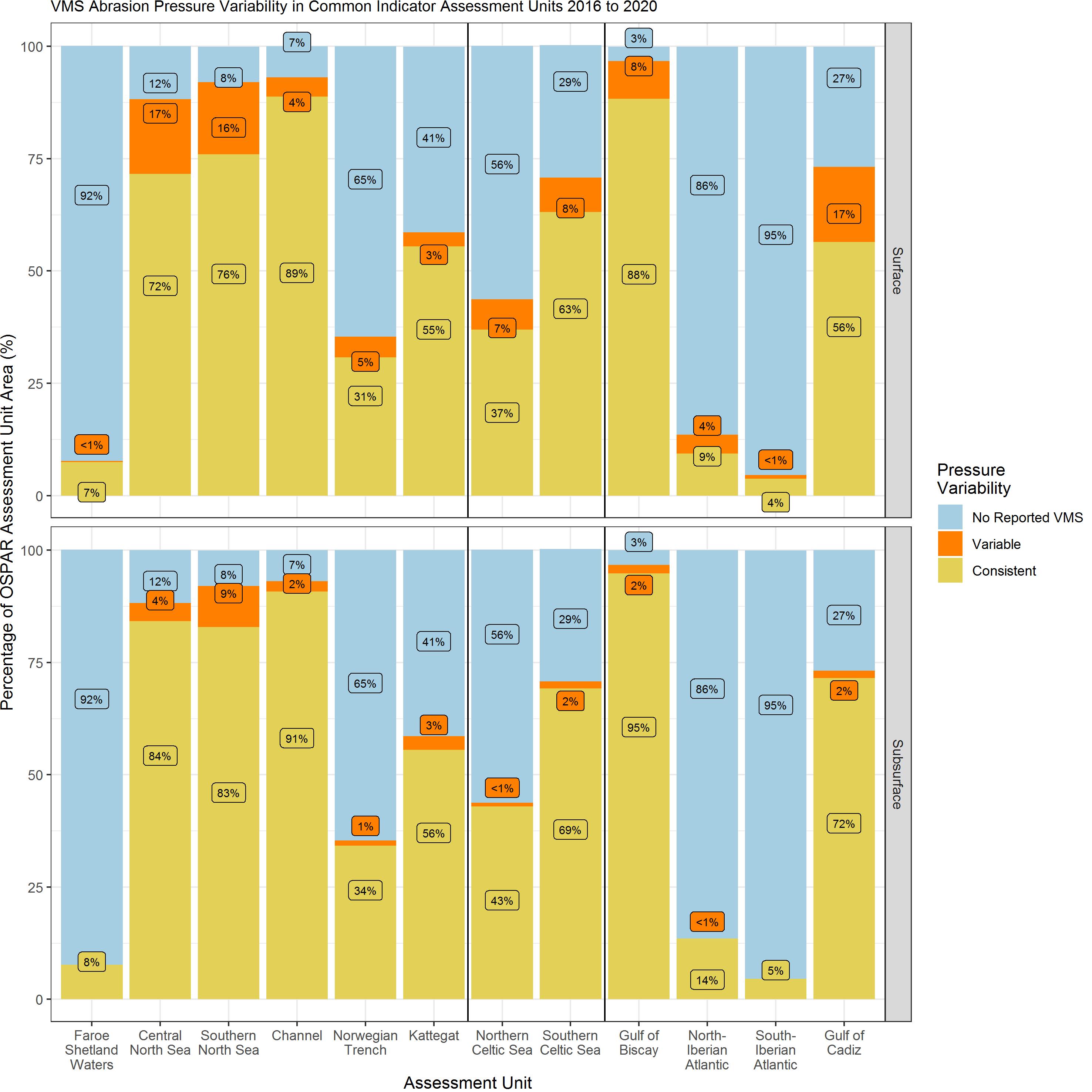
Figure y: Proportion of ‘Variable’, ‘Consistent’, and no VMS data in the assessment period 2016 to 2020. C-squares were categorised ‘Variable’ if a range of three or more SAR categories was observed throughout the time series
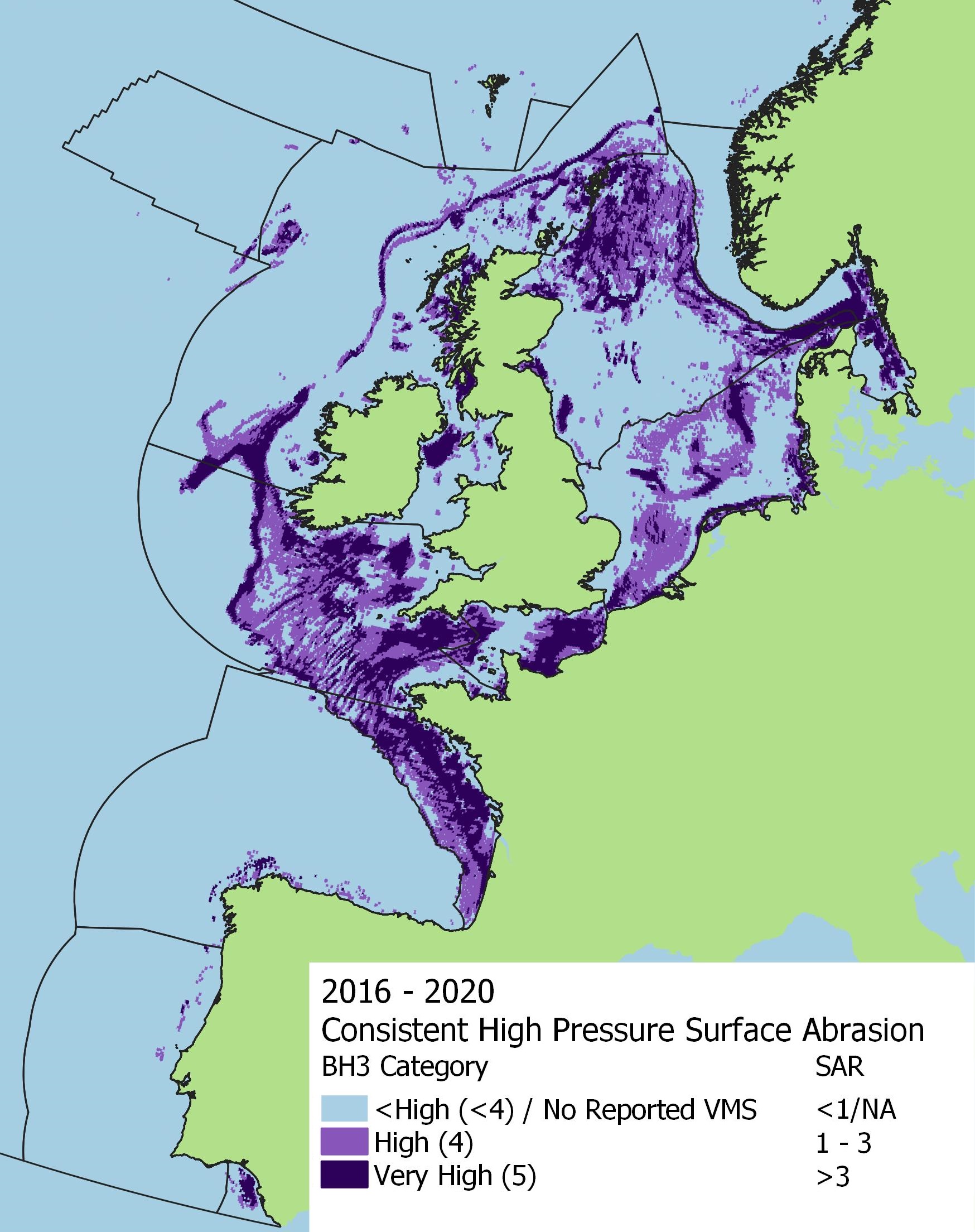
Figure z: Spatial distribution of consistently high (category 4 or 5) surface fishing pressure within the 2016 to 2020 assessment period. C-squares were considered to have ‘Consistent’ pressure if a change in less than three SAR categories was observed within the assessment period

Figure aa: Proportion of surface abrasion pressure categories in BHTs (excluding inconclusive translations) in the assessment period 2016 to 2020. 0* = 0 SAR value reported by ICES for vessels >12 m only. No EUNIS to BHT translation = EUNIS habitats that couldn’t be assigned MSFD translations (e.g., lacking substrate information); No EUNIS data = area of assessment unit where EUNIS habitat data were not available (habitat information unavailable or incompatible with EUNIS classification). The blue shading distinguishes between habitats of different biological zones, the red shading distinguishes No EUNIS data/No EUNIS to BHT translation from BHTs
The location and extent of areas with subsurface pressure categories of 3 or more in the 2016 to 2020 assessment period were similar to those categorised for 2009 to 2020 (Figure ab) and the proportion of subsurface abrasion categories in the assessment period 2016 to 2020 (Figure w) were also similar to those for 2009 to 2020. In addition, there was visibly less area of pressure categories 4 and 5 in the Fladen Grounds area of the Central North Sea and Cardigan Bay area of the Northern Celtic Sea in the 2016 to 2020, when compared with the 2009 to 2020 assessment (Figure w and Figure ab). It is possible that these differences in pressure category distribution between assessment periods were driven by higher intensity subsurface abrasion pressure before 2016 (therefore, only observed as high pressure in the 2009 to 2020 assessment).
Areas of variability in subsurface fishing pressure in the assessment period 2016 to 2020 (Figure ac) were notable in the Southern North Sea and Central North Sea (Figure y), whilst many areas with the highest subsurface abrasion categories were categorised as ‘Consistent’ (Figure ad). The assessment unit with the highest ‘Consistent’ values of subsurface abrasion was Gulf of Biscay (95%), closely followed by the Channel (91%) and Central and Southern North Sea (84% and 83% respectively).
Offshore circalittoral mud experienced subsurface pressure in more than 75% of the total assessment unit area across the 2016 to 2020 time period, with the exception of the Southern-Iberian Atlantic (Figure ae). In the Southern North Sea, Channel, Norwegian Trench and the Kattegat, more than 50% of the area of Offshore circalittoral mud experienced subsurface pressure categories 4 or 5. The Southern North Sea, Channel, Southern Celtic Sea, Kattegat, and Gulf of Biscay all showed multiple habitats with large proportions of subsurface pressure, including large proportions with subsurface pressure categories 4 and 5 (Figure ae).
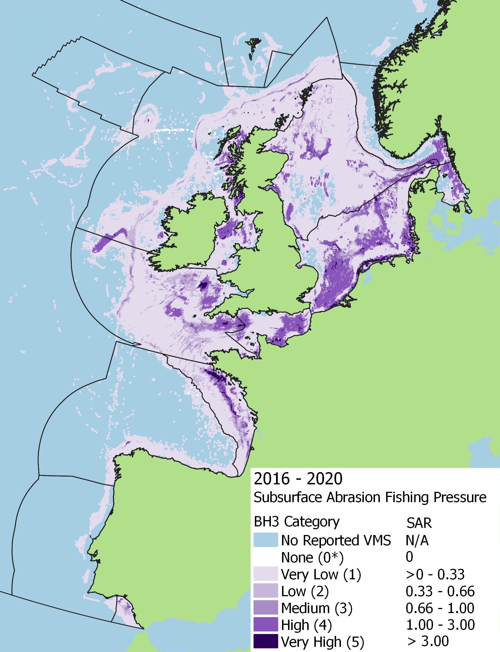
Figure ab: Aggregated subsurface abrasion pressure in the 2016 to 2020 assessment period. Note, BH3 category 0* = 0 SAR value reported by ICES for vessels >12 m only
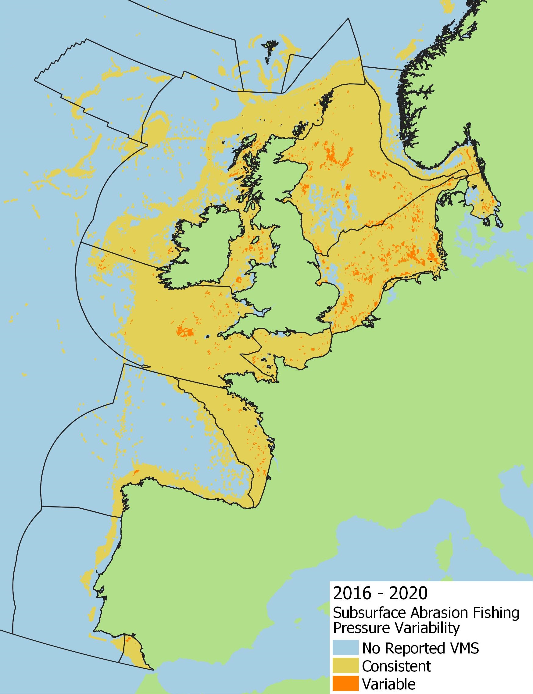
Figure ac: Spatial distribution of ‘Variable’ and ‘Consistent’ subsurface fishing pressure using the 2016 to 2020 assessment period. C-squares were categorised ‘Variable’ if a range of three or more SAR categories was observed throughout the time series
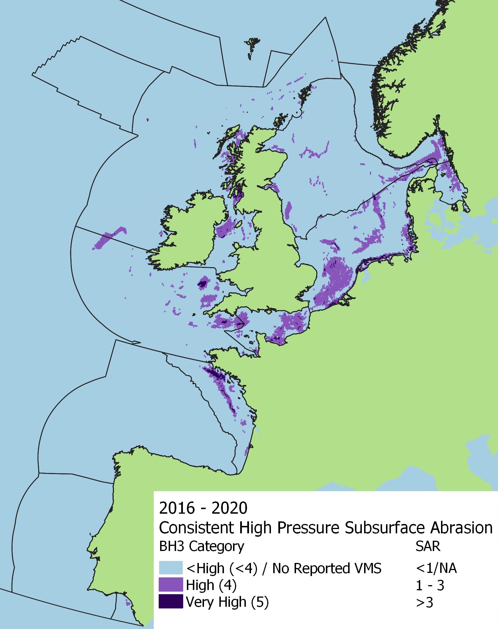
Figure ad: Spatial distribution of consistently high (category 4 or 5) subsurface fishing pressure within the 2009 to 2020 assessment period. C-squares were considered to have ‘Consistent’ pressure if a change in less than three SAR categories was observed within the assessment period
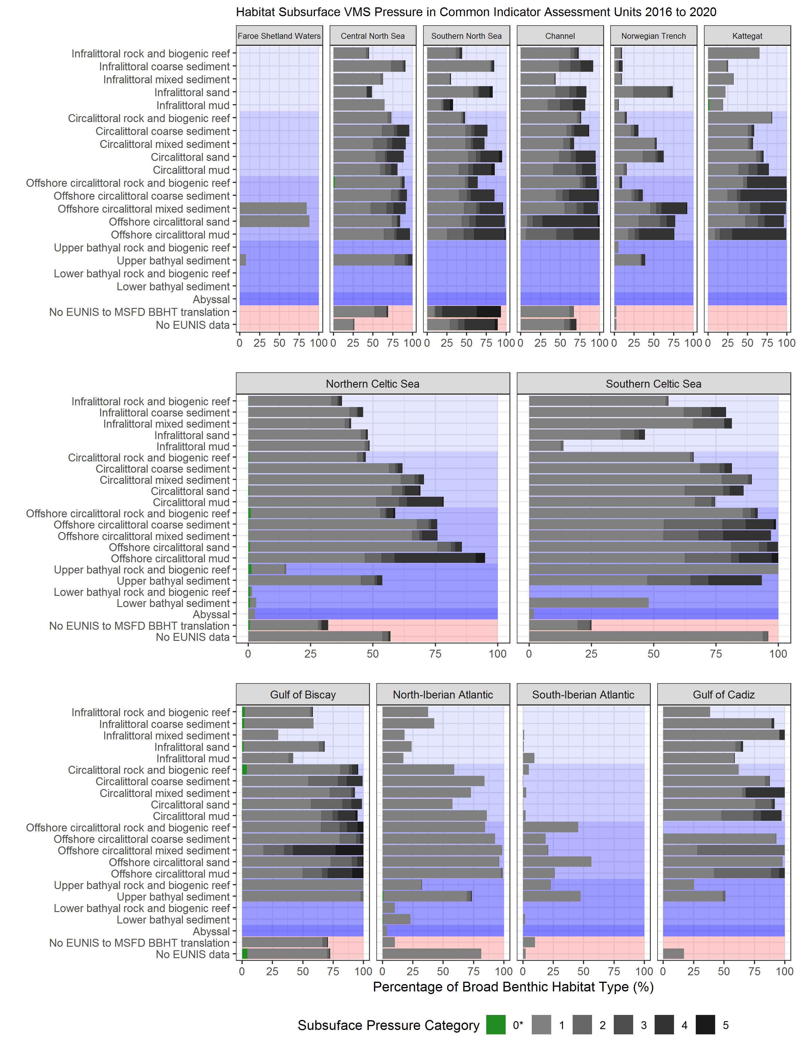
Figure ae: Proportion of subsurface abrasion pressure categories in BHTs (excluding inconclusive translations) in the assessment period 2016 to 2020. 0* = 0 SAR value reported by ICES for vessels >12 m only. No EUNIS to BHT translation = EUNIS habitats that couldn’t be assigned MSFD translations (e.g., lacking substrate information); No EUNIS data = area of assessment unit where EUNIS habitat data were not available (habitat information unavailable or incompatible with EUNIS classification). The blue shading distinguishes between habitats of different biological zones, the red shading distinguishes No EUNIS data/No EUNIS to BHT translation from BHTs
It should be noted that the surface and subsurface pressures maps (Figure l, Figure r, Figure v, and Figure ab) did not account for all bottom-contact fishing activity. Data were supplied by ICES (ICES, 2021) and some fleet data (Portugal, Iceland, and Norway) did not pass quality assurance checks required for inclusion in the data published by ICES; other fleet data (Faroe Islands, Greenland, and Russia) were not submitted. VMS data were supplied in the OSPAR Maritime Area, which did not include the Ise Fjord and Roskilde Fjord areas of the Kattegat assessment unit. Therefore, possible fishing pressure in this area could not be included in the BH3 QSR 2023 assessment. It was also expected that some pressure data may have been missing due to different approaches for extracting data from national databases. Data gaps also existed for fishing vessels with lengths less than 12 m and less than 15 m before 2012. This was an important consideration for inshore waters, where smaller vessels were most likely to operate. The inclusion of Inshore Vessel Monitoring Systems (I-VMS) data in future assessments would help address these knowledge gaps.
Fishing pressure in deep-sea areas
Overlaps were observed between deep-sea areas and those without VMS data (Figure l, Figure r, Figure v, Figure ab, and Figure af). Abyssal habitats occur below the continental shelf at depths greater than 2 000 m (EEA, 2016). Bottom contact fishing is banned at depths greater than 800 m in EU waters (Deep-Sea Access Restriction EU 2016 / 2336; retained in United Kingdom law via the Withdrawal Act 2018). Therefore, it was possible that deep-water areas that did not have VMS data were not suitable for bottom-contact fishing; pressure data in areas with known fishing closures likely had low confidence, and vessel speeds may have been slowed by extraneous variables, such as bad weather, rather than actual trawl activity. Pressure data, as provided by ICES, were not edited for transparency. However, disturbance calculations undertaken in the BH3 analyses adjusted disturbance outputs in areas with pressure data that had been identified as erroneous by experts across the OSPAR Maritime Area to 0 disturbance. These changes were made for Atlantic lower abyssal and Atlantic mid abyssal biological zones (derived from EUSeaMap2021) in the North-Iberian Atlantic.
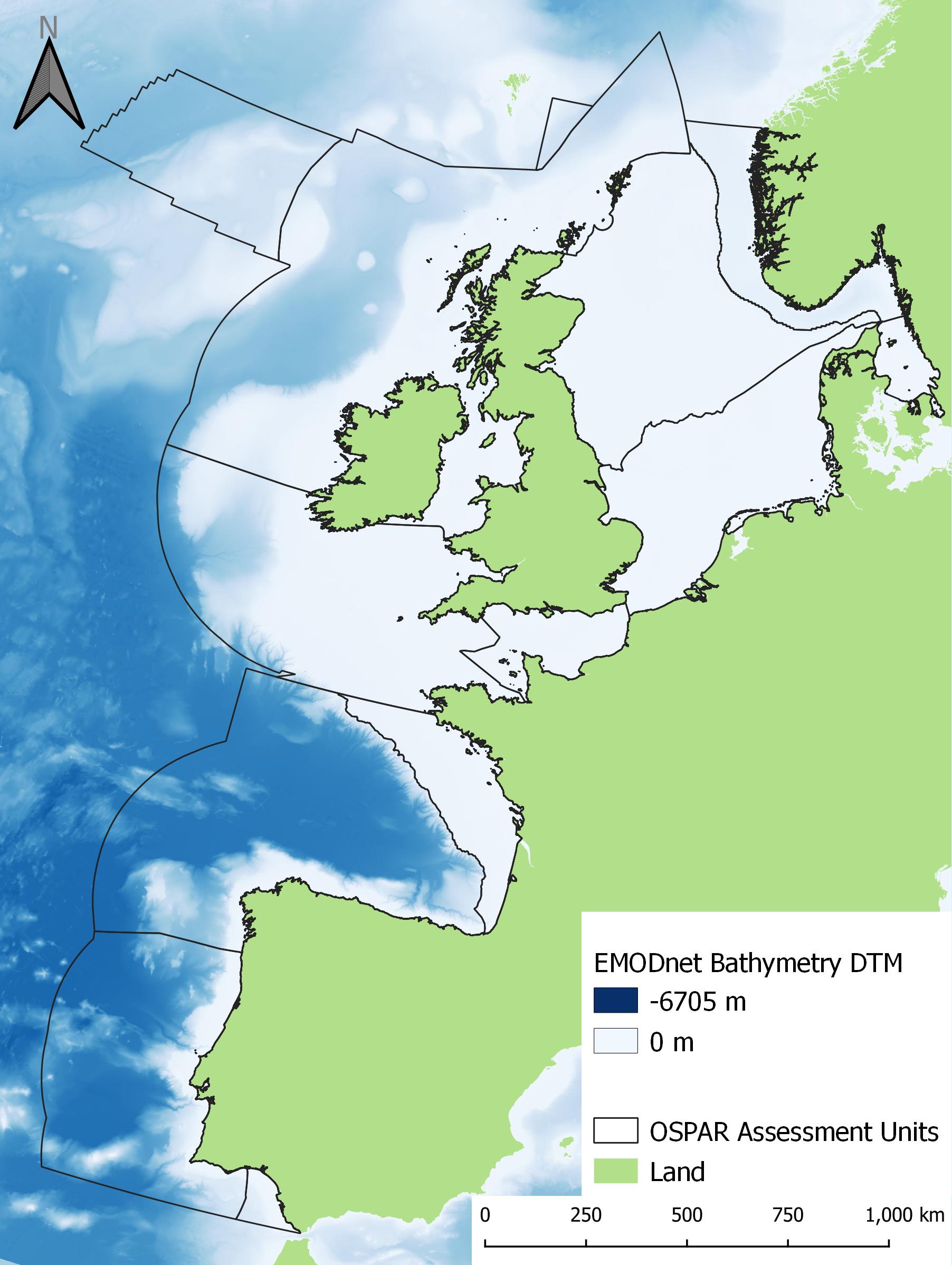
Figure af: EMODnet Bathymetry (EMODnet Bathymetry Consortium, 2020) across OSPAR assessment units where BH3 is a Common or Candidate Indicator
Seabed habitat disturbance
It should be noted that disturbance within the boundaries of MPAs in the United Kingdom was often higher than in surrounding areas beyond protected area boundaries, despite similar levels of pressure. Designated protected features within UK MPAs were mapped to EUNIS Level 3 (Figure b) and were therefore, only available at this resolution at the time of assessment. Following the precautionary approach of aggregating sensitivity from child biotopes, EUNIS Level 3 habitats were more likely to have higher sensitivity than more detailed biotope-resolution polygons (EUNIS Level 4-6) (Figure g and Figure h) and therefore, higher disturbance than adjacent areas of similar habitats mapped at EUNIS Level 4 and above. This caveat associated with available habitat data resulted in designated features appearing more sensitive than areas outside of protected area boundaries, which aligns with rationale for designation.
Total disturbance across Common Indicator Assessment units
2009 to 2020 assessment period
In the 2009 to 2020 assessment period, aggregated physical disturbance occurred in 53,0% of the total area of Common Indicator Assessment Units (see assessment method), where both pressure and sensitivity data were available (Table l). In the total assessed area of Common Indicator Assessment Units, 35,5% was ‘High’ and ‘Moderate’ disturbance (‘High’ 12,8% and ‘Moderate’ 22,7%). ‘Low’ disturbance covered 17,5% of total Common Indicator Assessment Unit Area and ‘Zero’ disturbance covered 44,9% of total Common Indicator Assessment Unit area (Figure 3, Table l). It should be noted that disturbance could not be assessed in 2,1% of the total area of Common Indicator Assessment Units where VMS data indicated pressure had occurred, due to an absence of underlying EUNIS habitat data and / or sensitivity information.
Table l: Percentage of total Common Indicator Assessment area under disturbance groups in the 2009 to 2020 assessment period where ‘Zero’ =disturbance category 0; ‘Low’ = disturbance categories 1-4; ‘Moderate’ = disturbance categories 5-7; ‘High’ = disturbance categories 8 and 9; ‘Unassessed Disturbance’ = area where fishing pressure was present but disturbance could not be assessed due to i) no habitat data, or ii) no sensitivity assessments for underlying habitat; ‘No VMS Data’ = area with no reported SAR values due to i) no fishing data submitted, or ii) habitat not suitable for fishing activities
| Disturbance Group | Percentage of total Common Indicator Assessment Area |
|---|---|
| Zero | 45,1% |
| Low | 17,4% |
| Moderate | 22,6% |
| High | 12,8% |
| Unassessed Disturbance | 2,1% |
Assessment Unit Summary: Faroe Shetland Waters
In total, disturbance occurred in 15% of the area of the Faroe Shetland Waters assessment unit (Figure as). ‘Moderate’ disturbance covered the largest proportion of the assessment unit (12%), followed by ‘High’ and ‘Low’ (3% and <1% respectively) (Figure as). The Highest disturbance occurred to the north-west of the Faroe Shetland Channel (Figure ag). Additionally, ‘Zero’ disturbance occurred throughout 84% of the assessment unit due to areas with no reported SAR values (Figure as). However, most of the assessment unit consisted of deep-sea habitats (Figure c) that were likely to not be suitable for bottom contact fishing.
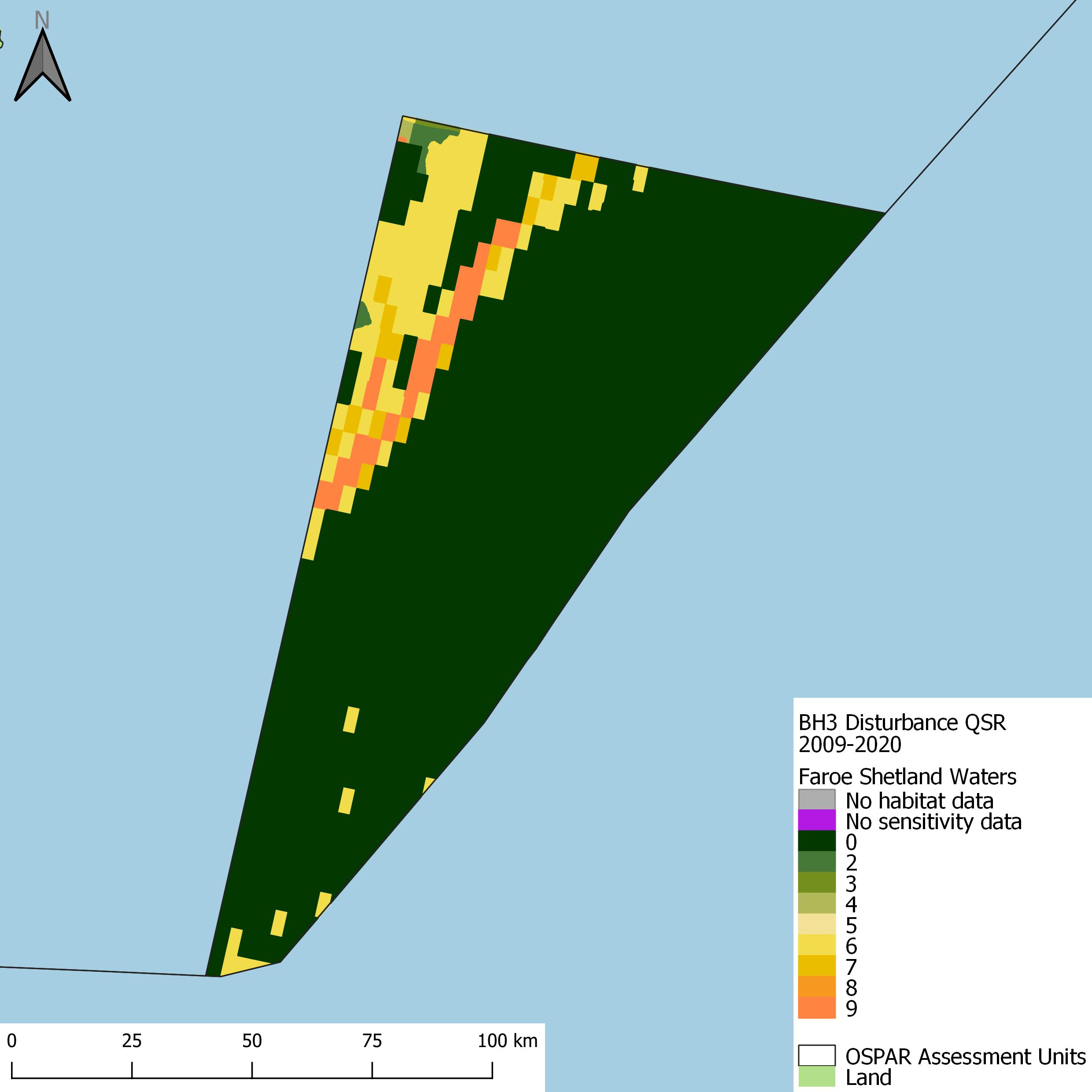
Figure ag: Spatial distribution of aggregated disturbance within Faroe Shetland Waters assessment unit in the 2009 to 2020 assessment period
Assessment Unit Summary: Central North Sea
The Central North Sea had the largest percentage of area covered by disturbance (95%) out of all 11 assessment units (Figure as). Out of the three disturbance groups, the greatest proportion of the assessment unit was covered by ‘Moderate’ disturbance (39%), followed by ‘Low’ (33%), and ‘High’ (23%) (Figure as). ‘Zero’ disturbance accounted for 5% of the assessment unit, predominantly in the southern part of the Central North Sea, north of Dogger Bank SAC (Figure ah). Areas with the highest levels of disturbance were south of the Shetland Islands, along the border with the Norwegian Trench assessment unit and the eastern and western borders of the Central North Sea assessment unit (Figure ah). The habitats with the largest proportions of area under ‘High’ disturbance were Upper bathyal sediment, followed by Offshore circalittoral mud (Figure au).
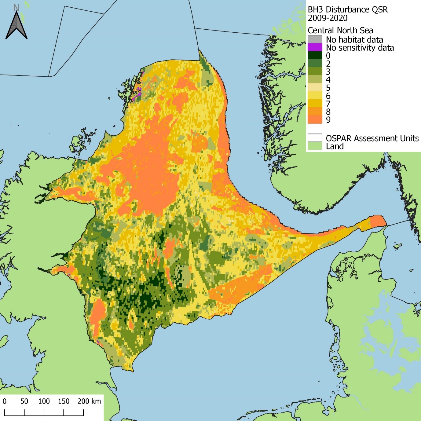
Figure ah: Spatial distribution of aggregated disturbance within the Central North Sea assessment unit in the 2009 to 2020 assessment period
Assessment Unit Summary: Southern North Sea
Disturbance occurred in 93% of the Southern North Sea, with the greatest proportion of area (53%) in ‘Moderate’ disturbance, followed by ‘Low’ disturbance (23%) and finally ‘High’ disturbance (23%) (Figure as). ‘Zero’ disturbance covered 5% of the area of the assessment unit (Figure as), located in the west of Dogger Bank SAC (Figure ai). Assessed disturbance was highest in the centre of the assessment unit, north of the Netherlands and east of Denmark, as well as in the south-east coast of England (Figure ai). The greatest proportion of area of habitat under ‘High’ disturbance was observed in Offshore circalittoral mud, followed by areas where EUNIS habitats could not be translated to BHT (Figure au). VMS data was absent from 5% of the assessment unit, predominantly off the coast of England and inshore areas around the Netherlands and Denmark (Figure ai and Figure as).
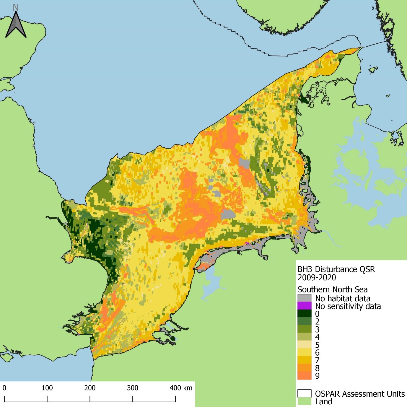
Figure ai: Spatial distribution of aggregated disturbance within the Southern North Sea assessment unit in the 2009 to 2020 assessment period
Assessment Unit Summary: Channel
The majority of the area of the Channel (94%) was assessed as disturbed, primarily as ‘Low’ disturbance (63%), followed by ‘Moderate’ (26%) and ‘High’ (5%) (Figure as). The highest categories of disturbance were located in areas south-east of the Isle of Wight, and in coastal areas of England and France (Figure aj). The percentage of the area of the Channel that had ‘Zero’ disturbance was 5%, comprising areas with no reported VMS, particularly around the Isle of Wight, Guernsey, Jersey, and the south-west of the assessment unit on the coast of Normandy (Figure aj and Figure as). ‘High’ disturbance was predominantly observed in Offshore circalittoral mud with most of its area under ‘High’ disturbance (Figure au).
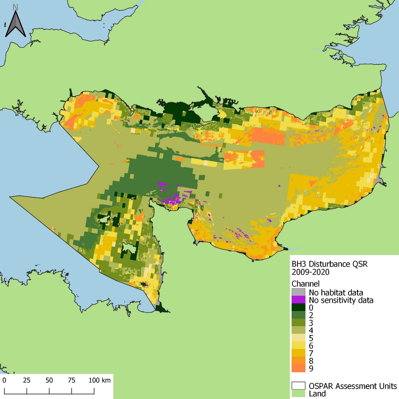
Figure aj: Spatial distribution of aggregated disturbance within the Channel assessment unit in the 2009 to 2020 assessment period
Assessment Unit Summary: Norwegian Trench
In total, 42% of the area of the Norwegian Trench assessment unit had disturbance, with the majority of disturbance being ‘Moderate’ (23%), followed by ‘High’ (17%) and ‘Low’ (1%) (Figure as). The highest disturbance occurred along the border of the assessment unit with the Central North Sea, and in the Skagerrak (Figure ak). Additionally, 58% of the Norwegian Trench had ‘Zero’ disturbance, predominantly along coastal Norway, and Sweden and within the Swedish No Trawl Zone. Offshore circalittoral mud had the majority of area under ‘High’ disturbance, followed by Upper bathyal sediment (Figure au). VMS data were not reported for 32% of the assessment unit area, largely along the coastline with Norway (Figure ak).
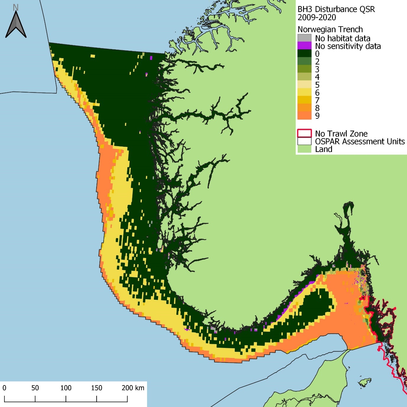
Figure ak: Spatial distribution of aggregated disturbance within the Northern Trench assessment unit in the 2009 to 2020 assessment period
Assessment Unit Summary: Kattegat
Disturbance covered 61% of the Kattegat assessment unit, the majority of the area under disturbance was classified as ‘High’ (26%), followed by ‘Low’ (23%) and ‘Moderate’ (12%) (Figure as). High disturbance was predominantly observed in the centre of the assessment unit, running alongside the border with the Swedish No Trawl Zone. Of the total area, 39% had ‘Zero’ disturbance, predominantly within the Swedish No Trawl Zone, Ålborg bay and Ise Fjord areas of the assessment unit, due to a lack of VMS data and the presence of the Swedish No Trawl Zone. The proportion of habitat area under ‘High’ disturbance was greatest in Offshore circalittoral mud, Circalittoral mud and Circalittoral mixed sediment (Figure au). Just under one third of the assessment unit was lacking VMS data (32%) particularly coastal Denmark and Sweden, and Ålborg bay (Figure al and Figure as). The Swedish habitat data is only allowed to be used in a low resolution in regional assessments due to national security reasons. Furthermore, VMS data were supplied for the OSPAR Maritime Area which did not include the Ise Fjord and Roskilde Fjord areas of the Kattegat assessment unit.
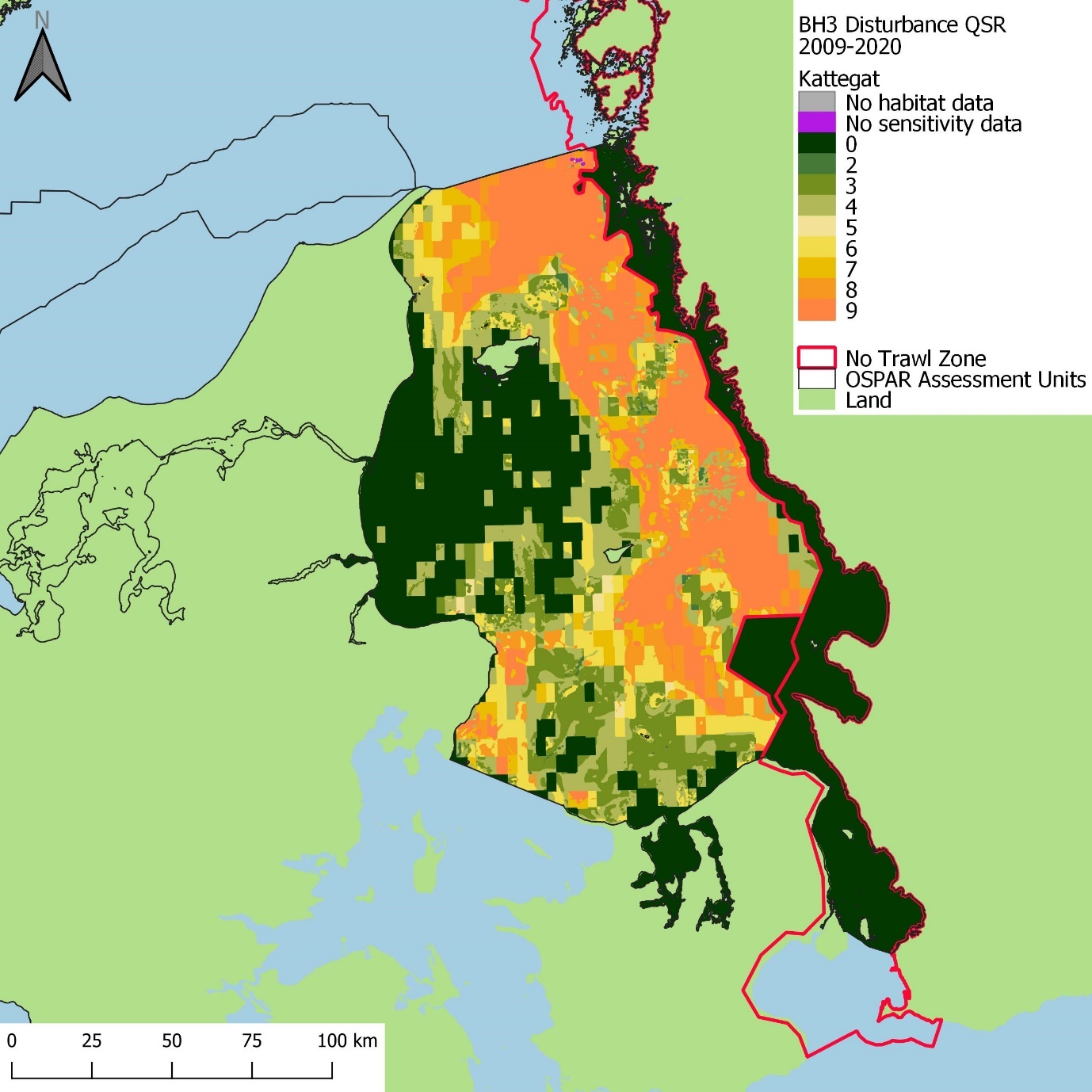
Figure al: Spatial distribution of aggregated disturbance within the Kattegat assessment unit in the 2009 to 2020 assessment period
Assessment Unit Summary: Northern Celtic Sea
Less than half (48%) of the Northern Celtic Sea was assessed as having disturbance, mostly under ‘Low’ disturbance (19%), followed by ‘Moderate’ (15%) and ‘High’ (14%). Areas including the north of the Irish Sea off the coast of Northern Ireland, the Firth of Clyde, the Hebrides, Rockall Bank, and the boundary of the continental shelf experienced the highest disturbance (Figure am). Just under half (48%) of the Northern Celtic Sea had ‘Zero’ disturbance, due solely to VMS data paucity, primarily around the coasts of the Republic of Ireland, Northern Ireland, Wales and England, the Rockall Plateau, and the north and west of the assessment unit (Figure am). Offshore circalittoral mud had the largest proportion of area under ‘High’ disturbance, followed by Upper bathyal sediment (Figure au).
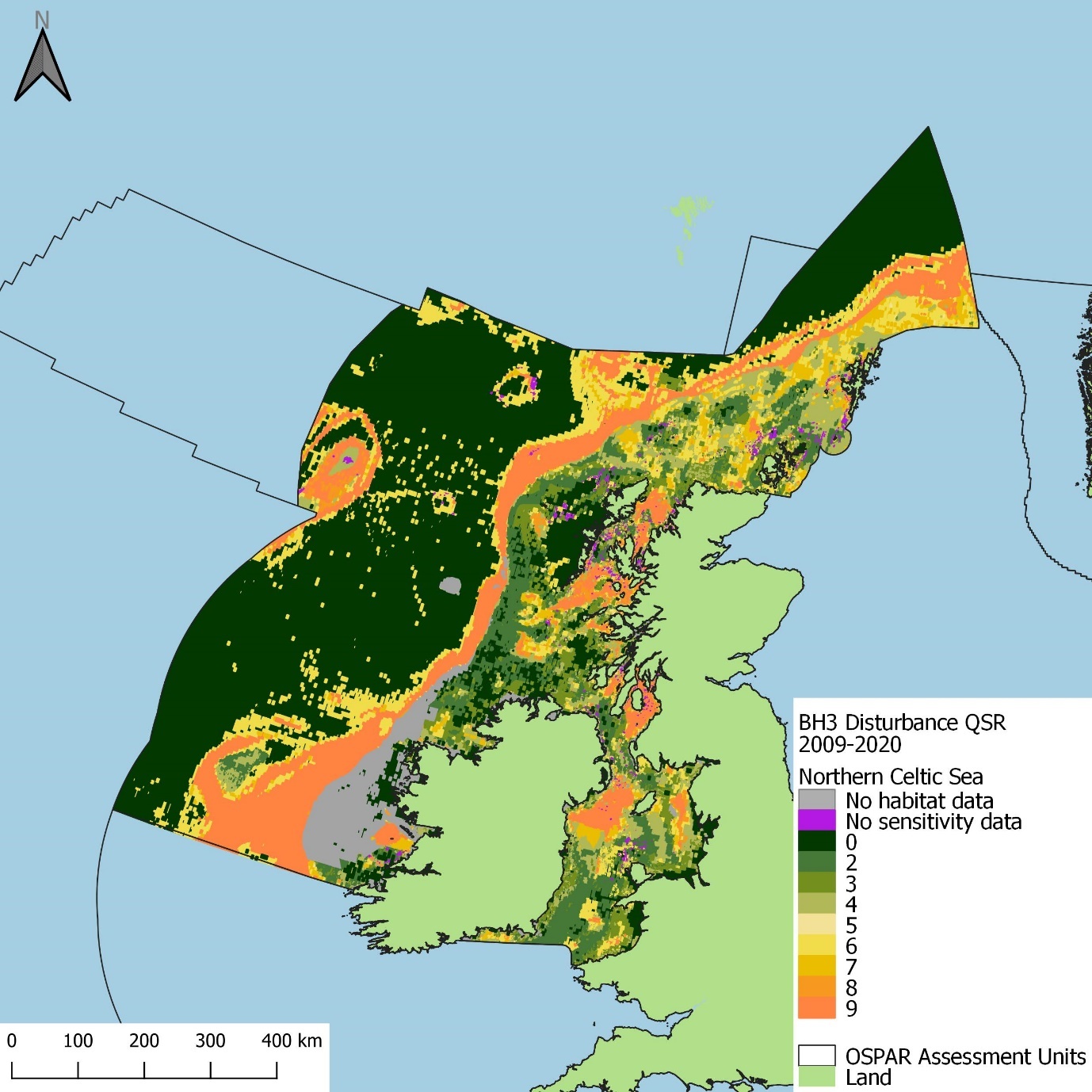
Figure am: Spatial distribution of aggregated disturbance within the Northern Celtic Sea assessment unit in the 2009 to 2020 assessment period
Assessment Unit Summary: Southern Celtic Sea
Disturbance in the Southern Celtic Sea occurred throughout 73% of the assessment unit area; ‘Moderate’ disturbance was the greatest proportion (33%), followed by ‘Low’ (24%) and ‘High’ (16%). ‘Zero’ disturbance occurred in 24% of the area of the Southern Celtic Sea, due solely to VMS data paucity, predominantly in areas beyond the continental shelf, inshore areas south-west coast of Ireland, the Bristol Channel, and inshore areas of France (Figure an). Highest disturbance in the assessment unit was located south-west of Skomer, off the southern coast of Ireland and the boundary of the assessment unit with the North-Iberian Atlantic and along the boundary of the continental shelf (Figure an). The habitat with the greatest proportion of area under ‘High’ disturbance was Offshore circalittoral mud, followed by Upper bathyal sediment (Figure au).
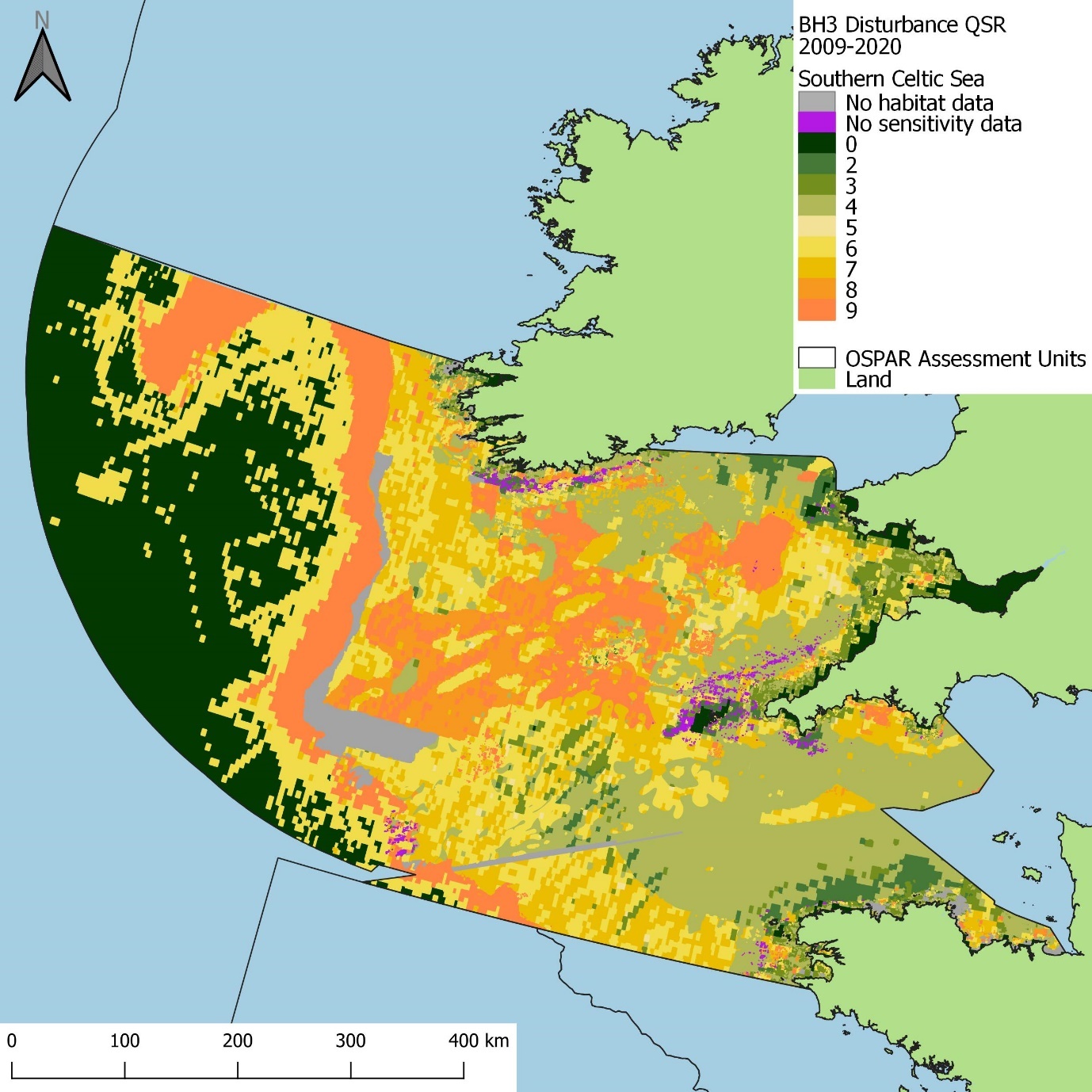
Figure an: Spatial distribution of aggregated disturbance within the Southern Celtic Sea assessment unit in the 2009 to 2020 assessment period
Assessment Unit Summary: Gulf of Biscay
Disturbance was present throughout 94% of the Gulf of Biscay assessment unit (Figure as), with highest disturbance occurring along the Armoricain shelf and in the north-west portion of the assessment unit, bordering the North-Iberian Atlantic assessment unit (Figure ao). Nearly half of the assessment unit was under ‘Moderate’ disturbance (48%) followed by ‘Low’ (24%) and ‘High’ (22%) (Figure as). Of the Gulf of Biscay assessment unit area, 3% had ‘Zero’ disturbance, as a result of VMS data paucity only, largely around inshore areas of France. Offshore circalittoral mud had the greatest proportion of area under ‘High’ disturbance, followed by Upper bathyal sediment (Figure au). The Gulf of Biscay had the most complete coverage of VMS data out of all assessment units.
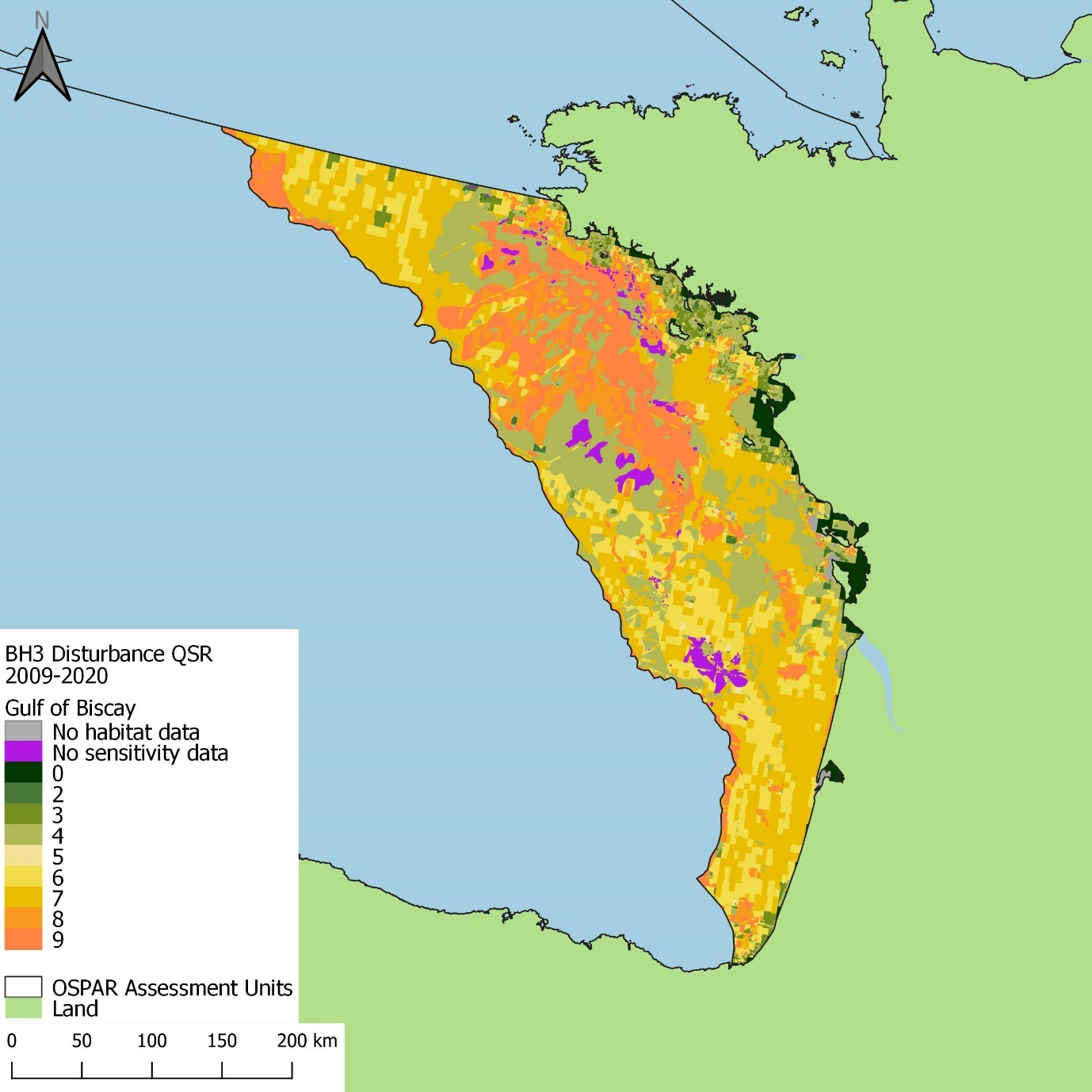
Figure ao: Spatial distribution of aggregated disturbance within the Gulf of Biscay assessment unit in the 2009 to 2020 assessment period
Assessment Unit Summary: North-Iberian Atlantic
In total, 13% of the North-Iberian Atlantic assessment unit area had disturbance, with ‘Moderate’ disturbance covering 7% of the assessment unit, followed by ‘High’ (4%) and ‘Low’ (2%) (Figure as). ‘Zero’ disturbance occurred in 87% of the North-Iberian Atlantic assessment unit, due to a combination of amendments to the disturbance results where Atlantic lower abyssal and Atlantic mid abyssal biological zones were present, and VMS data availability. Areas under the highest disturbance were located off the Spanish coast and along the border with the Gulf of Biscay assessment unit (Figure ap). Offshore circalittoral mud had the greatest proportion of area under ‘High’ disturbance, followed by Upper bathyal sediment. VMS data were not available in the majority of the assessment unit (83%), particularly in deeper areas beyond the continental shelf (Figure ap).
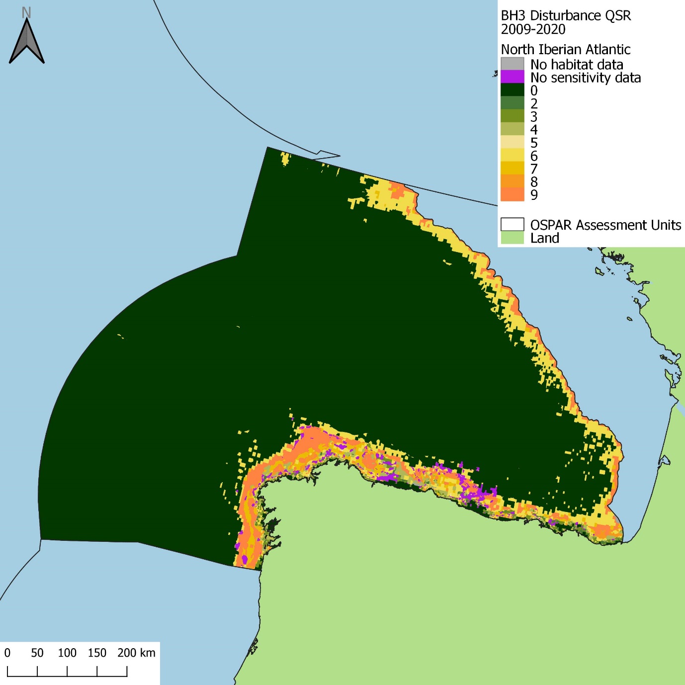
Figure ap: Spatial distribution of aggregated disturbance within the North Iberian Atlantic assessment unit in the 2009 to 2020 assessment period
Assessment Unit Summary: South-Iberian Atlantic
In comparison with other assessment units, The South-Iberian Atlantic had the smallest percentage of area with disturbance (5%), although it should be noted that this was largely due to data paucity, where 94% of the assessment unit was not covered by VMS data (Figure as), and therefore classed as ‘Zero’ disturbance. The greatest proportion of disturbance in the South-Iberian Atlantic was ‘Moderate’ disturbance (3%) with ‘High’ and ‘Low’ disturbance both at 1% (Figure as). Disturbance was predominantly located along the margin of the continental shelf, with the highest disturbance towards the north of the assessment unit (Figure aq). Upper bathyal sediment had the largest percentage area under ‘High’ disturbance, followed by Offshore circalittoral mud (Figure au).
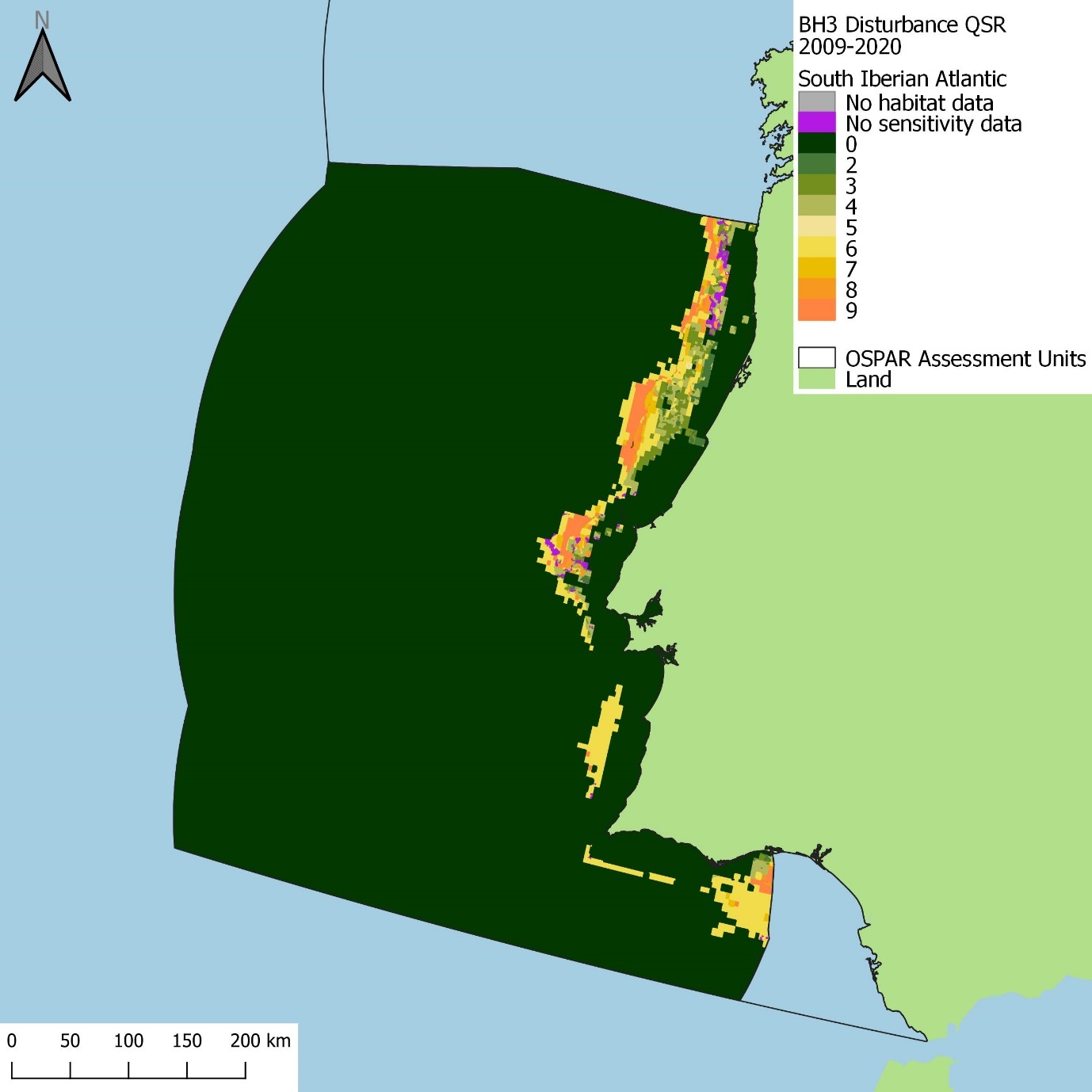
Figure aq: Spatial distribution of aggregated disturbance within the South Iberian Atlantic assessment unit in the 2009 to 2020 assessment period
Assessment Unit Summary: Gulf of Cadiz
The Gulf of Cadiz had the greatest percentage area under ‘High’ disturbance for any assessment unit (32%) (Figure as). In combination with ‘Low’ and ‘Moderate’ disturbance groups (both covering 20% of the assessment unit), 72% of the Gulf of Cadiz was under disturbance (Figure as). Disturbance was predominantly located towards the Spanish coast, with higher disturbance in the north of the assessment unit (Figure ar). ‘Zero’ disturbance occurred in 26% of the Gulf of Cadiz, as a result of VMS data paucity alone. Offshore circalittoral mud and Circalittoral mixed sediment were the habitats with the largest proportions of area with ‘High’ disturbance (Figure au). VMS data coverage was missing in 26% of the area of the assessment unit, mainly in deeper areas beyond the continental shelf and the strait of Gibraltar (Figure ar).
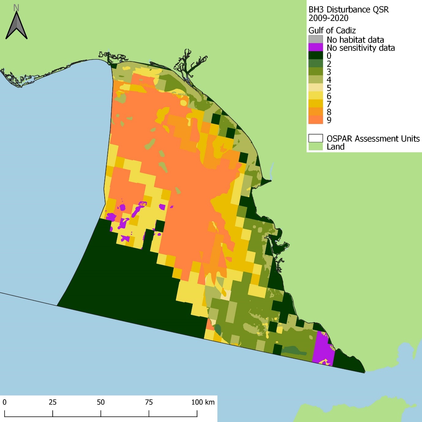
Figure ar: Spatial distribution of aggregated disturbance within the Gulf of Cadiz assessment unit in the 2009 to 2020 assessment period
Percentage of assessment unit area in each disturbance group
In the 2009 to 2020 assessment period, the proportion of assessment unit area in each disturbance group varied (Figure as). The greatest percentage of ‘High’ and ‘Moderate’ disturbance combined (70%) was in the Gulf of Biscay (‘High’ 22% and ‘Moderate’ 48%), followed closely by the Southern North Sea (69%; ‘High’ 16% and ‘Moderate’ 53%), Central North Sea (62%; ‘High’ 23% and ‘Moderate’ 39%), Gulf of Cadiz (52%; ‘High’ 32% and ‘Moderate’ 20%), and Southern Celtic Sea (49%; ‘High’ 16% and ‘Moderate’ 33%) (Figure as).
When considering the occurrence of disturbance groups within assessment units individually, the greatest percentage of ‘High’ disturbance was observed in the Gulf of Cadiz (32%) (Figure as), which was predominantly distributed in the northwest of the assessment unit (Figure ar). Conversely, the Channel had the greatest percentage of area with ‘Low’ disturbance, which covered close to two thirds (63%) of the assessment unit, predominantly in western and central areas (Figure aj and Figure as).
Despite the large area of ‘Low’ disturbance in the Channel, there were greater percentages of pressure categories 4 and 5 than were observed in the Gulf of Cadiz (Figure m). Therefore, the differences in disturbance between the two locations was the direct result of more sensitive habitats coinciding with higher intensities of pressure. For example, the Gulf of Cadiz contained a greater percentage of area with sensitivity categories 4 and 5; 100% of Offshore circalittoral mud had a surface / subsurface sensitivity score of 4 (Figure j and Figure k), covering 11% of the total assessment unit area (Figure f) and was predominantly covered by very high surface pressure (5) (Figure l, Figure m and Figure q), resulting in the observed ‘High’ levels of disturbance (Figure as). In contrast, habitats in the Channel mainly had sensitivity categories of 2 and 3, resulting in lower disturbance, despite higher levels of pressure. For example, Offshore circalittoral coarse sediment and circalittoral mixed sediment collectively covered 65% of the Channel and predominantly had sensitivities of 2 and 3, respectively (Figure f and Figure i to Figure k).
The greatest percentage of area with ‘Zero’ disturbance was observed in the South-Iberian and North-Iberian Atlantic (94% and 87% respectively; Figure as), predominantly in offshore waters off the coast of Spain and Portugal. The assessment units with the least percentage of area with ‘Zero’ disturbance were the Central and Southern North Sea, the Channel, and the Gulf of Biscay (all 5% or less; Figure as).
Due to aforementioned data limitations, it was not possible to distinguish whether areas without VMS were always true representations of ‘Zero’ disturbance from fishing activity. This was especially the case in assessment units where fleet data were not reported (e.g., from Norway and Portugal), although it was expected that these missing fleets active. However, where it was likely that fishing did not occur, such as waters deeper than 800 m (where bottom-contact fishing is banned); (Deep-Sea Access Restriction EU 2016 / 2336), representations of ‘Zero’ disturbance had higher confidence (Figure af).
Figure as: The percentage of OSPAR Common indicator assessment unit area under each of the following disturbance groups in the 2009 to 2020 assessment period: ‘Zero’ = disturbance category 0; ‘Low’ = disturbance categories 1-4; ‘Moderate’ = disturbance categories 5-7; ‘High’ = disturbance categories 8 and 9; ‘Unassessed Disturbance’ = area where fishing pressure was present but disturbance could not be assessed due to i) no habitat data, or ii) no sensitivity assessments for underlying habitat
Habitat disturbance across assessment units
When disturbance was analysed within the total area of each habitat across all assessment units (where BH3 is agreed as a Common Indictor), all 20 distinct BHTs had ‘High’ and / or ‘Moderate’ disturbance throughout the 2009 to 2020 assessment period (Figure at). Additionally, six habitats (30% of BHTs), ranging from the Infralittoral to the Offshore circalittoral zone, had more than, or equal to 50% of their area in ‘Moderate’ and / or ‘High’ disturbance (Infralittoral mixed sediment, Circalittoral mud, Circalittoral sand, Upper bathyal sediment, Offshore circalittoral sand, and Offshore circalittoral mud) (Figure at). However, Offshore circalittoral mud was the only habitat where more than 50% of its area was in ‘High’ disturbance alone (87%). ‘Moderate’ disturbance was recorded in over 50% of the total area of Offshore circalittoral sand (73%) and Circalittoral sand (57%). ‘Low’ disturbance was greatest in areas with Offshore circalittoral coarse sediment (91%), closely followed by Offshore circalittoral mixed sediment (79%) and Infralittoral coarse sediment (62%) (Figure at).
All 20 distinct BHTs had areas of ‘Zero’ disturbance, from 98% of the habitat area across all Common Indicator Assessment Units in Abyssal, to 4% in Offshore circalittoral sand and Offshore circalittoral mud (Figure at). ‘Zero’ disturbance was recorded in over 50% of the area of seven BHTs: Abyssal (98%), Lower bathyal sediment (87%), Lower bathyal rock and biogenic reef (85%), Upper bathyal rock and biogenic reef (70%), Infralittoral mud (57%), Infralittoral rock and biogenic reef (53%), and Infralittoral mixed sediment (51%).
Figure at: The percentage of each distinct BHT’s area across OSPAR Common Indicator Assessment Units under each of the following disturbance groups in the 2009 to 2020 assessment period: ‘High’ = disturbance categories 8 and 9; ‘Moderate’ = disturbance categories 5-7; ‘Low’ = disturbance categories 1-4; ‘Zero’ disturbance category 0; and ‘Unassessed Disturbance’ = area where fishing pressure was present but disturbance could not be assessed due to i) no habitat data, or ii) no sensitivity assessments for underlying habitat
Habitats with the greatest proportions of area without VMS data comprised Abyssal and Lower bathyal biological zones, therefore, the absence of VMS data may have been attributed to reduced fishing in deep-sea areas due to trawl bans in depths greater than 800 m (Deep-Sea Access Restriction EU 2016 / 2336) (Figure u and Figure aa). However, it should be noted that disturbance values may have been underestimated in other habitats that may have had poor VMS data coverage. This may have affected Infralittoral habitats, in particular, due to aforementioned limitations such as a lack of data from vessels under 12 m in length and areas where fleets not reported in the data may be active.
Disturbance within habitat types within Common Indicator Assessment Units
‘High’ and / or ‘Moderate’ disturbance groups were not observed in all distinct BHTs when analysing habitat disturbance within Common Indicator Assessment Units. When analysing habitats in assessment units individually, 15 of 20 distinct BHTs (75% of BHTs) had ‘High’ and / or ‘Moderate’ disturbance in all Common Indicator Assessment Units they occurred in (Table m). The 15 habitats ranged from Infralittoral to Abyssal zones, with particular prevalence in the Circalittoral zone, where all habitats had ‘High’ and / or ‘Moderate’ disturbance in all Common Indicator Assessment Units they occurred in. ‘High’ and / or ‘Moderate’ disturbance was also observed in all assessment units where EUNIS to BHT translations were not possible; this resulted from translating from disturbance calculated at EUNIS Levels 2-6 to BHT, which had reduced resolution of habitat detail. In addition, four BHTs (20%), ranging from Circalittoral to Bathyal zones, had ‘High’ disturbance in all assessment units they occurred in (Table m). Mud habitats were particularly affected as both Circalittoral and Offshore circalittoral mud had ‘High’ disturbance in all Common Indicator Assessment Units in which they occurred.
Furthermore, Offshore circalittoral mud had the greatest proportion of ‘High’ disturbance across nine of the 11 Common Indicator Assessment Units in the 2009 to 2020 assessment period (Figure au). In the South-Iberian Atlantic and the Central North Sea, the greatest proportions of ‘High’ disturbance occurred in Upper bathyal sediment (Figure au). Although Offshore circalittoral mud contained the greatest proportion of ‘High’ disturbance across the total area of Common Indicator Assessment Units (Figure at), in the South-Iberian Atlantic lower levels of disturbance were observed due to reduced surface pressure intensity and coverage within the habitat (Figure q). In the Central North Sea, the percentage of ‘High’ disturbance in Offshore circalittoral mud aligned with other assessment units, but a greater proportion of ‘High’ disturbance was observed in Upper bathyal sediment due to a combination of increased pressure intensity and coverage (Figure q). However, this was likely due to Upper bathyal sediment covering a relatively small area of the Central North Sea (<1%) (Figure f).
Table m: The presence of ‘High’ (disturbance categories 8 and 9) and ‘Moderate’ (disturbance categories 5-7) disturbance groups within habitats across OSPAR benthic assessment units the habitat occurs in, where BH3 is agreed as Common, in the 2009 to 2020 assessment period. Blue shading indicates the biological zone of the habitat; ticks indicate that the disturbance group was present across all assessment units the habitat occurred in; crosses indicate the disturbance group was not present in all assessment units that the habitat occurred in
| BHT | High and/or Moderate | High |
|---|---|---|
| Infralittoral rock and biogenic reef | ü | û |
| Infralittoral coarse sediment | û | û |
| Infralittoral mixed sediment | ü | û |
| Infralittoral sand | ü | û |
| Infralittoral mud | ü | û |
| Circalittoral rock and biogenic reef | ü | û |
| Circalittoral coarse sediment | ü | û |
| Circalittoral mixed sediment | ü | ü |
| Circalittoral sand | ü | û |
| Circalittoral mud | ü | ü |
| Offshore circalittoral rock and biogenic reef | ü | û |
| Offshore circalittoral coarse sediment | û | û |
| Offshore circalittoral mixed sediment | û | û |
| Offshore circalittoral sand | ü | û |
| Offshore circalittoral mud | ü | ü |
| Upper bathyal rock and biogenic reef | û | û |
| Upper bathyal sediment | ü | ü |
| Lower bathyal rock and biogenic reef | û | û |
| Lower bathyal sediment | û | û |
| Abyssal | ü | û |
| No EUNIS to MSFD BBHT translation | ü | û |
| No EUNIS data | û | û |
Figure au: The percentage of BHT area in each OSPAR Common Indicator Assessment Unit under each of the following disturbance groups in the 2009 to 2020 assessment period: ‘Zero’ = disturbance category 0; ‘Low’ = disturbance categories 1-4; ‘Moderate’ = disturbance categories 5-7; ‘High’ = disturbance categories 8 and 9; ‘Unassessed Disturbance’ = area where fishing pressure was present but disturbance could not be assessed due to i) no habitat data, or ii) no sensitivity assessments for underlying habitat. Horizontal black lines represent the separation in biological zones
Offshore circalittoral sand had the greatest percentage of habitat area with ‘Moderate’ disturbance across assessment units, with the exception of the Gulf of Cadiz (Figure au), where Offshore circalittoral sand had predominantly ‘Low’ disturbance. The sensitivity of Offshore circalittoral sand was consistent across assessment units (Figure j and Figure k), therefore, ‘Low’ disturbance in the Gulf of Cadiz was predominantly driven by lower reported surface pressure intensity over Offshore circalittoral sand.
Both Offshore circalittoral coarse sediment and Offshore circalittoral mixed sediment had large percentages of ‘Low’ disturbance across Common Indicator Assessment Units (Figure au). Offshore circalittoral coarse sediment had the greatest percentage of area with ‘Low’ disturbance in eight of the 11 Common Indicator Assessment Units (Central North Sea, Southern North Sea, the Channel, Kattegat, Northern Celtic Sea, Southern Celtic Sea, North Iberian Atlantic, South Iberian Atlantic). Offshore circalittoral mixed sediment had the greatest percentage of area with ‘Low’ disturbance in two of the 11 Common Indicator Assessment Units (Norwegian Trench and Gulf of Cadiz). In the Gulf of Biscay, the percentage of ‘Low’ disturbance was equal in both Offshore circalittoral coarse sediment and Offshore circalittoral mixed sediment.
Abyssal and Infralittoral mixed sediment habitats had large percentages of ‘Zero’ disturbance within Common Indicator Assessment Units (Figure au). Abyssal had the greatest percentage of area with ‘Zero’ disturbance in three of the 11 Common Indicator Assessment Units (Northern Celtic Sea, North-Iberian Atlantic and Southern Celtic Sea). Infralittoral mixed sediment had the greatest percentage of area with ‘Zero’ disturbance in two of the 11 Common Indicator Assessment Units (the Channel and the Gulf of Biscay). The BHTs with the largest percentage of area with ‘Zero’ disturbance all differed in the remaining six Common Indicator Assessment Units but ranged from Lower bathyal to Infralittoral biological zones.
In the Gulf of Cadiz, where the greatest percentage of ‘High’ disturbance was observed, ‘High’ disturbance covered more than 90% of Circalittoral mixed sediment and Offshore circalittoral mud, and over 50% of Circalittoral mud. However, Circalittoral mixed sediment covered a relatively small area of the Gulf of Cadiz (1%), while Circalittoral mud and Offshore circalittoral mud both covered more than 10% of the assessment unit, respectively (Figure f). Therefore, Circalittoral mud and Offshore circalittoral mud made greater contributions to the large percentage of ‘High’ disturbance in the Gulf of Cadiz.
In the Channel, where the greatest proportion of ‘Low’ disturbance was observed, ‘Low’ disturbance covered more than 90% of Offshore circalittoral coarse sediment, and over 50% of Offshore circalittoral rock and biogenic reef, Offshore circalittoral mixed sediment and Infralittoral coarse sediment (Figure au). Offshore circalittoral mud was the only habitat in the Channel with the majority of its area under ‘High’ disturbance (over 90%). However, Offshore circalittoral mud had a very low extent of coverage in the Channel (less than 1%) (Figure f), meaning that this would have had little effect on the overall disturbance recorded in the assessment unit.
2016 to 2020
Total disturbance across Common Indicator Assessment Units
In the 2016 to 2020 assessment period, physical disturbance occurred in 48,3% of the total area of Common Indicator Assessment Units, where both pressure and sensitivity data were available (Table n). In the total area of Common Indicator Assessment Units, 30,3% was ‘High’ and ‘Moderate’ disturbance (‘High’ 11,0% and Moderate 19,3%). ‘Low’ disturbance covered 18.0% of total Common Indicator Assessment Unit area and ‘Zero’ disturbance (SAR values of 0 in VMS data, where VMS data were not reported, and where the associated biological zone was Atlantic lower abyssal and Atlantic mid abyssal in the North-Iberian Atlantic) covered 49,9% of total Common Indicator Assessment Unit area (Figure 3, Table n).
As observed in the 2009 to 2020 assessment, disturbance could not be assessed in 1,8% of the total area of Common Indicator Assessment Units where VMS data indicated pressure had occurred, due to an absence of underlying EUNIS habitat data and / or sensitivity information. Almost half (49,9%) of the total area of Common Indicator Assessment Units did not contain VMS data (due to data gaps or habitats not being suitable for fishing), and therefore, were assigned a disturbance group of ‘Zero’. However, it was possible that the absence of VMS in 49,9% of the total area of Common Indicator Assessment Units resulted from the reduction in total VMS data analysed over the shorter timeframe (rather than a reduction in the extent of fishing activity).
Table n: Percentage of total Common Indicator Assessment area under disturbance groups in the 2016 to 2020 assessment period where ‘Zero’ = disturbance category 0; ‘Low’ = disturbance categories 1-4; ‘Moderate’ = disturbance categories 5-7; ‘High’ = disturbance categories 8 and 9; ‘Unassessed Disturbance’ = area where fishing pressure was present but disturbance could not be assessed due to i) no habitat data, or ii) no sensitivity assessments for underlying habitat
| Disturbance Group | Percentage of total Common Indicator Assessment Area |
|---|---|
| Zero | 50,1% |
| Low | 18,0% |
| Moderate | 19,2% |
| High | 10,9% |
| Unassessed Disturbance | 1,8% |
Assessment Unit Summary: Faroe Shetland Waters
In total, disturbance occurred in ~6% of the area of the Faroe Shetland Waters assessment unit (Figure bh). ‘Moderate’ disturbance covered the largest proportion of the assessment unit (6%), followed by ‘High’ and ‘Low’ (both <1%) (Figure bh). The highest disturbance occurred to the northwest of the assessment unit, along the Faroe Shetland Channel (Figure av). Additionally, ‘Zero’ disturbance occurred throughout 92% of the assessment unit due to areas with no reported SAR values (Figure bh). However, most of the assessment unit consisted of deep-sea habitats (Figure c) that were likely to not be suitable for bottom-contact fishing.
Figure av: Spatial distribution of aggregated disturbance within Faroe Shetland Waters assessment unit in the 2016 to 2020 assessment period
Assessment Unit Summary: Central North Sea
In total, 89% of the area of the Central North Sea had disturbance (Figure bh). Highest disturbance was predominantly south of the Shetland Islands, along the border with the Norwegian Trench assessment unit and the eastern and western fringes of the assessment unit (Figure aw). Disturbance groups ‘Moderate’ and ‘Low’ comprised the greatest percentages of the assessment unit (both 34%) followed by ‘High’ (21%) (Figure bh). ‘Zero’ disturbance occurred in 12% of the area of the Central North Sea, as a result of VMS data paucity alone, primarily in the south-east and coastal fringes of England and Scotland (Figure aw and Figure bh). The habitats predominantly under ‘High’ disturbance were Offshore circalittoral mud and Upper bathyal sediment habitats (Figure bj).
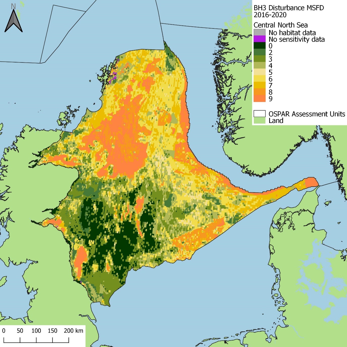
Figure aw: Spatial distribution of aggregated disturbance within the Central North Sea assessment unit in the 2016 to 2020 assessment period
Assessment Unit Summary: Southern North Sea
In total, 89% of the Southern North Sea assessment unit area had disturbance (Figure bh). Highest disturbance was predominantly located in the centre of the assessment unit, north of the Netherlands and east of Denmark (Figure ax). The majority of the area (45%) was assessed as ‘Moderate’ disturbance, followed by ‘Low’ (31%) and ‘High’ (13%) (Figure bh). ‘Zero’ disturbance occurred in 8% of the Southern North Sea, due to VMS data paucity alone, predominantly in coastal areas located off the East of England, and some areas along the western coast of Denmark (Figure ax and Figure bh). ‘High’ disturbance was predominantly observed in Offshore circalittoral mud and in areas where EUNIS habitats could not be translated to MSFD (Figure bj).
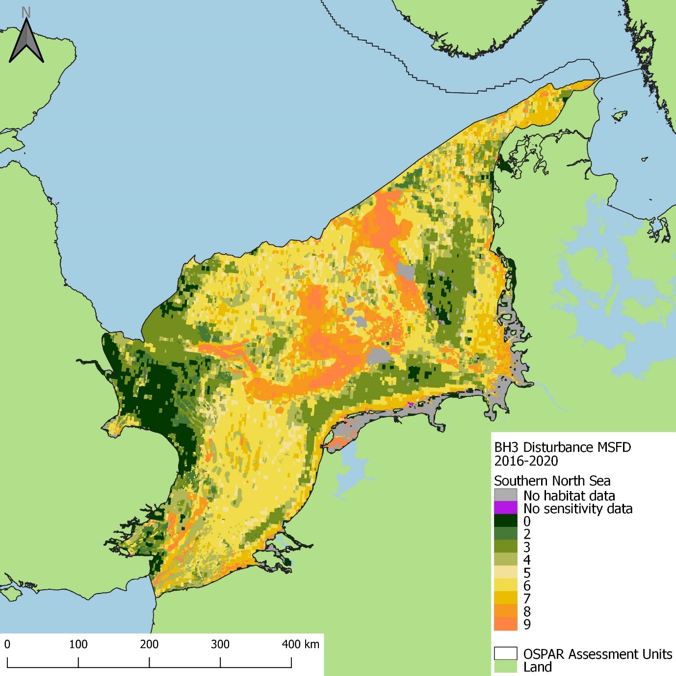
Figure ax: Spatial distribution of aggregated disturbance within the Southern North Sea assessment unit in the 2016 to 2020 assessment period
Assessment Unit Summary: Channel
The majority of the Channel assessment unit had disturbance (92% of assessment unit area, Figure bh). The highest levels of disturbance were observed offshore off the south coast of England, east of Offshore Overfalls MCZ and in patchy locations off the coast of the south-east of England (Figure ay). Most of the Channel had ‘Low’ disturbance (64% of the assessment unit area) followed by ‘Moderate’ (24%) and ‘High’ (4%) (Figure bh). ‘Zero’ disturbance occurred in 7% of the Channel due to VMS data paucity, predominantly around the Isle of Wight, Guernsey, Jersey, and the south-west of the assessment unit near the coast of Normandy (Figure ay and Figure bh). Habitats with the largest proportions under ‘High’ disturbance were Offshore circalittoral mud and Offshore circalittoral rock and biogenic reef (Figure bj).
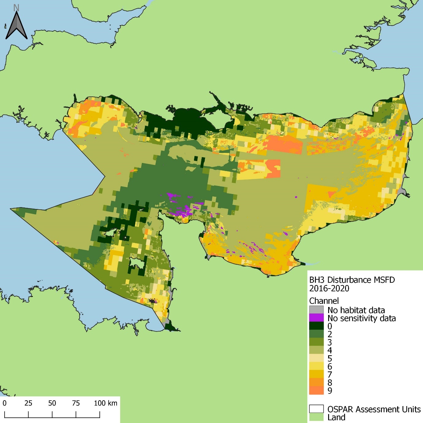
Figure ay: Spatial distribution of aggregated disturbance within the Channel assessment unit in the 2016 to 2020 assessment period
Assessment Unit Summary: Norwegian Trench
Disturbance covered 34% of the Norwegian Trench assessment unit area (Figure bh); ‘Moderate’ disturbance covered the largest proportion (18%), followed by ‘High’ (15%) and ‘Low’ (1%). The highest disturbance was located in the Skagerrak and along the border with the Central North Sea assessment unit (Figure az). Additionally, 65% of the Norwegian Trench had ‘Zero’ disturbance, predominantly along coastal Norway, and Sweden and within the Swedish No Trawl Zone. The habitats within the Norwegian Trench assessment unit with the highest percentages of area under ‘High’ disturbance were Offshore circalittoral mud and Upper bathyal sediment (Figure bj). VMS data were not available for 65% of the assessment unit, particularly along the coastline of Norway (Figure az and Figure bh).
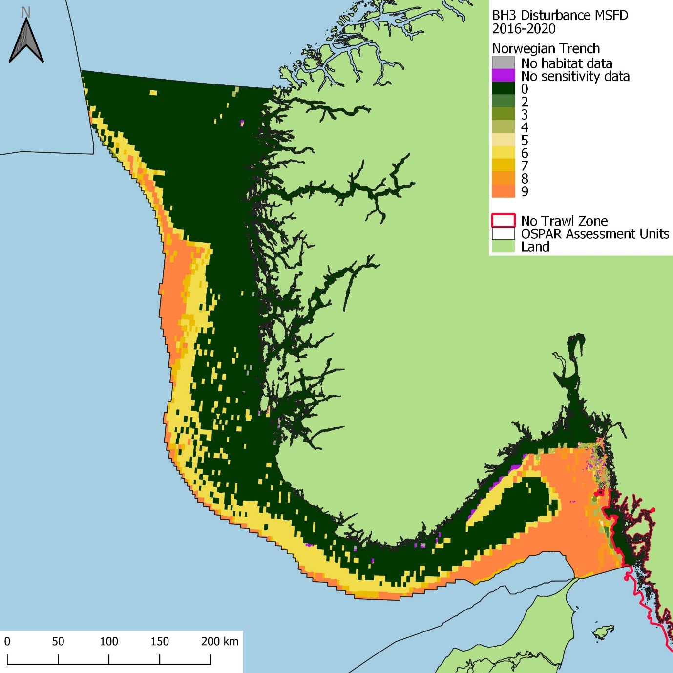
Figure az: Spatial distribution of aggregated disturbance within the Norwegian Trench assessment unit in the 2016 to 2020 assessment period
Assessment Unit Summary: Kattegat
Disturbance covered 54% of the Kattegat assessment unit area, comprising ‘High’ (25%), ‘Low’ (19%), and ‘Moderate’ (10%) disturbance groups (Figure bh). Disturbance was predominantly observed in the centre of the assessment unit, running alongside the border with the Swedish No Trawl Zone (Figure ba). Of the total area, 47% had ‘Zero’ disturbance, predominantly within the Swedish No Trawl Zone, Ålborg bay and Ise Fjord areas of the assessment unit, due to a lack of VMS data and the presence of the Swedish No Trawl Zone. Habitats in the Kattegat with the greatest proportions of area with ‘High’ disturbance were Offshore circalittoral mud, followed by Circalittoral mud (Figure bj). VMS data were not available for 41% of the assessment unit area, located largely around coastal Denmark and Sweden, and Ålborg bay (Figure ba and Figure bh). The Swedish habitat data is restricted to a low resolution in regional assessments due to national security reasons. Habitat data could be improved in the future or in national assessments using the BH3 method. Furthermore, VMS data were supplied for the OSPAR Maritime Area, which did not include the Ise Fjord and Roskilde Fjord areas of the Kattegat assessment unit.
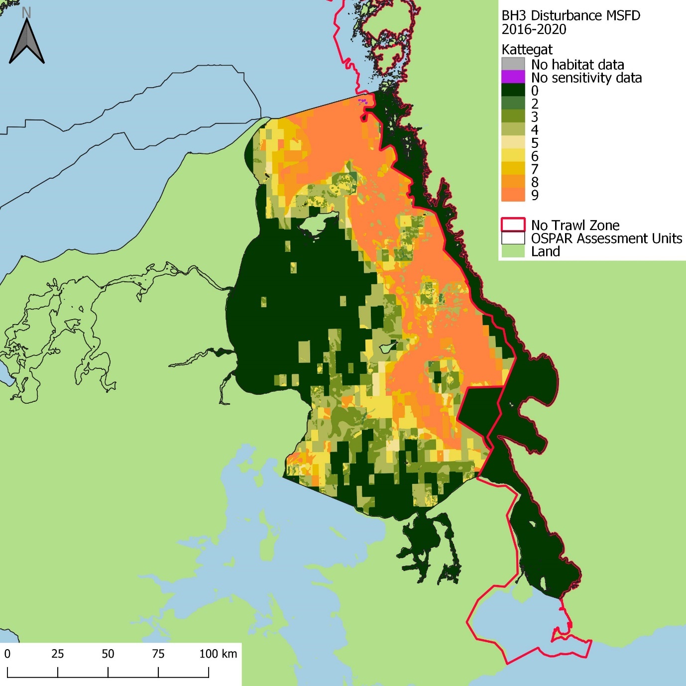
Figure ba: Spatial distribution of aggregated disturbance within the Kattegat assessment unit in the 2016 to 2020 assessment period
Assessment Unit Summary: Northern Celtic Sea
In total, 41% of the area of the Northern Celtic Sea assessment unit had disturbance (Figure bh). ‘Low’ disturbance covered the largest proportion of the assessment unit (17%), followed by ‘High’ and ‘Moderate’ (both 12% of the area) (Figure bh). The highest disturbance was found in the north of the Irish Sea off the coast of Northern Ireland, the Firth of Clyde, the Hebrides, Rockall Bank, and along the boundaries continental shelf (Figure bb). Additionally, ‘Zero’ disturbance occurred throughout 56% of the assessment unit due to a combination of the presence of c-squares with a SAR value of 0, and of VMS data paucity. Habitats with the greatest proportions of their area under ‘High’ disturbance included Offshore circalittoral mud, followed by Upper bathyal sediment, and Circalittoral mixed sediment (Figure bj). VMS data was not available in 56% of the assessment unit area, in particular along the coast of Wales and England, the Rockall Plateau and the north and west of the assessment unit (Figure bb and Figure bh), and contributed to the large proportion of ‘Zero’ disturbance in this Northern Celtic Sea.
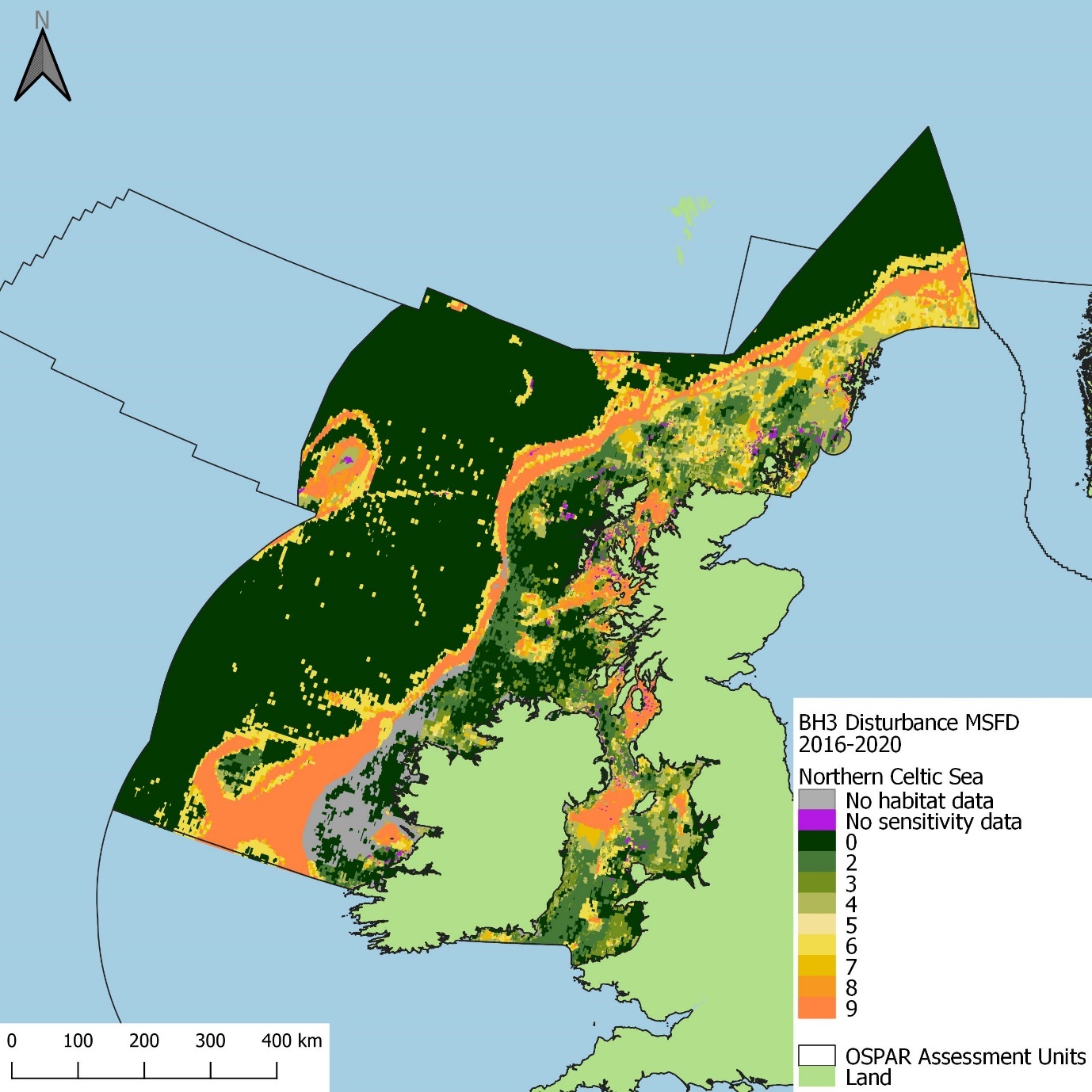
Figure bb: Spatial distribution of aggregated disturbance within the Northern Celtic Sea assessment unit in the 2016 to 2020 assessment period
Assessment Unit Summary: Southern Celtic Sea
In total, 68% of the Southern Celtic Sea area had disturbance (Figure bh); ‘Moderate’ disturbance covered the greatest percentage (28%) of area, followed by ‘Low’ (26%) and ‘High’ (14%) (Figure bh). ‘High’ disturbance was primarily located the south-west of Skomer, south of the southern coast of Ireland and along the boundary of the continental shelf (Figure bc). ‘Zero’ disturbance occurred in 29% of the Southern Celtic Sea, due to VMS data paucity alone, located largely in the Bristol Channel and Rockall Trough (Figure bc and Figure bh). Habitats with the largest proportions of area under ‘High’ disturbance included Offshore circalittoral mud, followed by Upper bathyal sediment (Figure bj).
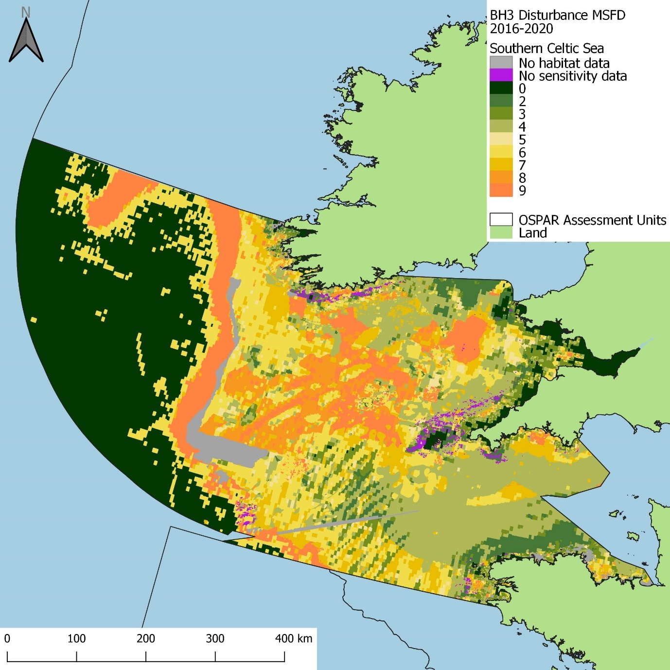
Figure bc: Spatial distribution of aggregated disturbance within the Southern Celtic Sea assessment unit in the 2016 to 2020 assessment period
Assessment Unit Summary: Gulf of Biscay
In comparison with other assessment units the Gulf of Biscay had the highest percentage of area with disturbance (94%) (Figure bh). ‘Moderate’ disturbance had the largest coverage of the assessment unit area (46%), followed by ‘Low’ (27%) and ‘High’ (21%) (Figure bh). The highest categories of disturbance were located along the Armoricain shelf and the western boundary of the assessment unit (Figure bd). ‘Zero’ disturbance occurred in 3% of the area of the Gulf of Biscay, due to VMS data paucity, located along the coastline of France (Figure bd and Figure bh). Habitats with the largest percentages of area under ‘High’ disturbance included Offshore circalittoral mud, followed by Upper bathyal sediment and Circalittoral mixed sediment (Figure bj).
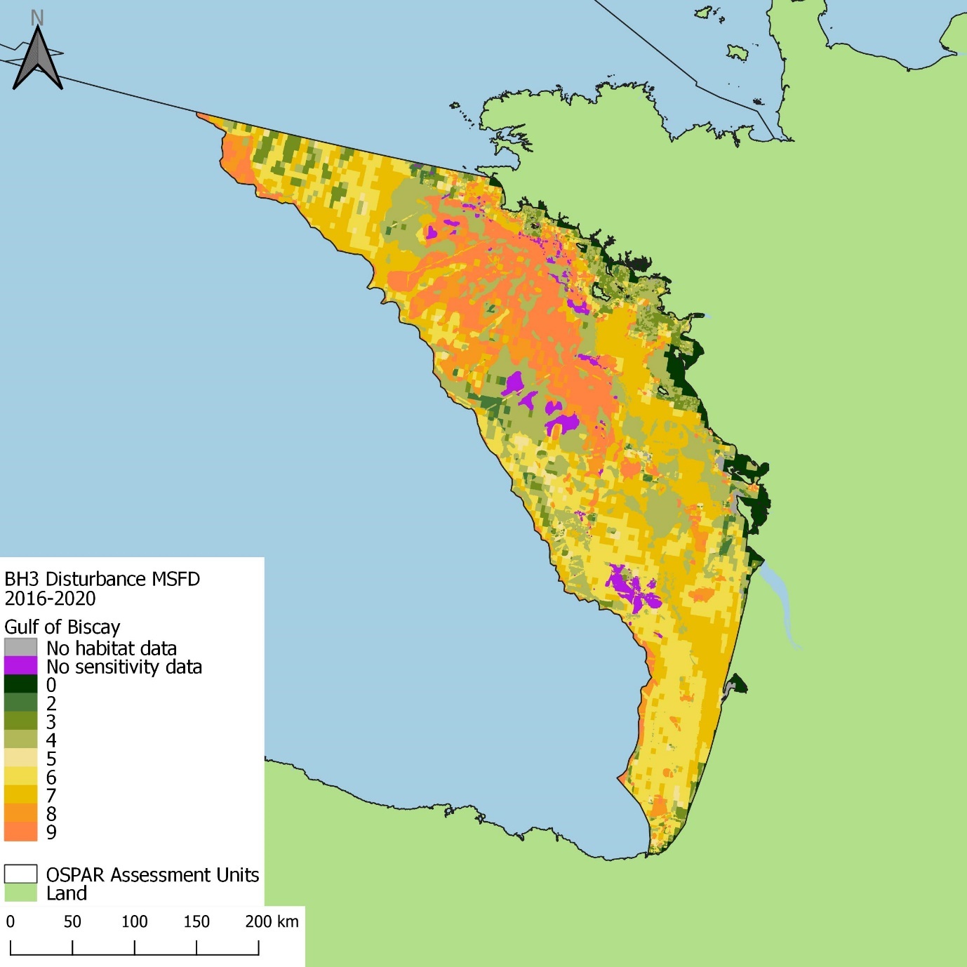
Figure bd: Spatial distribution of aggregated disturbance within the Gulf of Biscay assessment unit in the 2016 to 2020 assessment period
Assessment Unit Summary: North-Iberian Atlantic
In total, 10% of the North-Iberian Atlantic assessment unit area had disturbance; the category with the greatest coverage was ‘Moderate’ disturbance (6%), followed by ‘High’ (3%) and ‘Low’ (1%) (Figure bh). Highest disturbance categories were situated along the north coast of Spain and the border with the Gulf of Biscay assessment unit (Figure be). ‘Zero’ disturbance occurred in 89% of the North-Iberian Atlantic assessment unit, due to a combination of amendments to the disturbance results where Atlantic lower abyssal and Atlantic mid abyssal biological zones were present, and VMS data availability. Offshore circalittoral mud, followed by Upper bathyal sediment, and Circalittoral mixed sediment were the habitats that had the greatest percentages of area under ‘High’ disturbance in the North-Iberian Atlantic (Figure bj). VMS data were not available for 86% of the North-Iberian Atlantic assessment unit, with gaps predominantly in offshore, deep-water areas (Figure be and Figure bh).
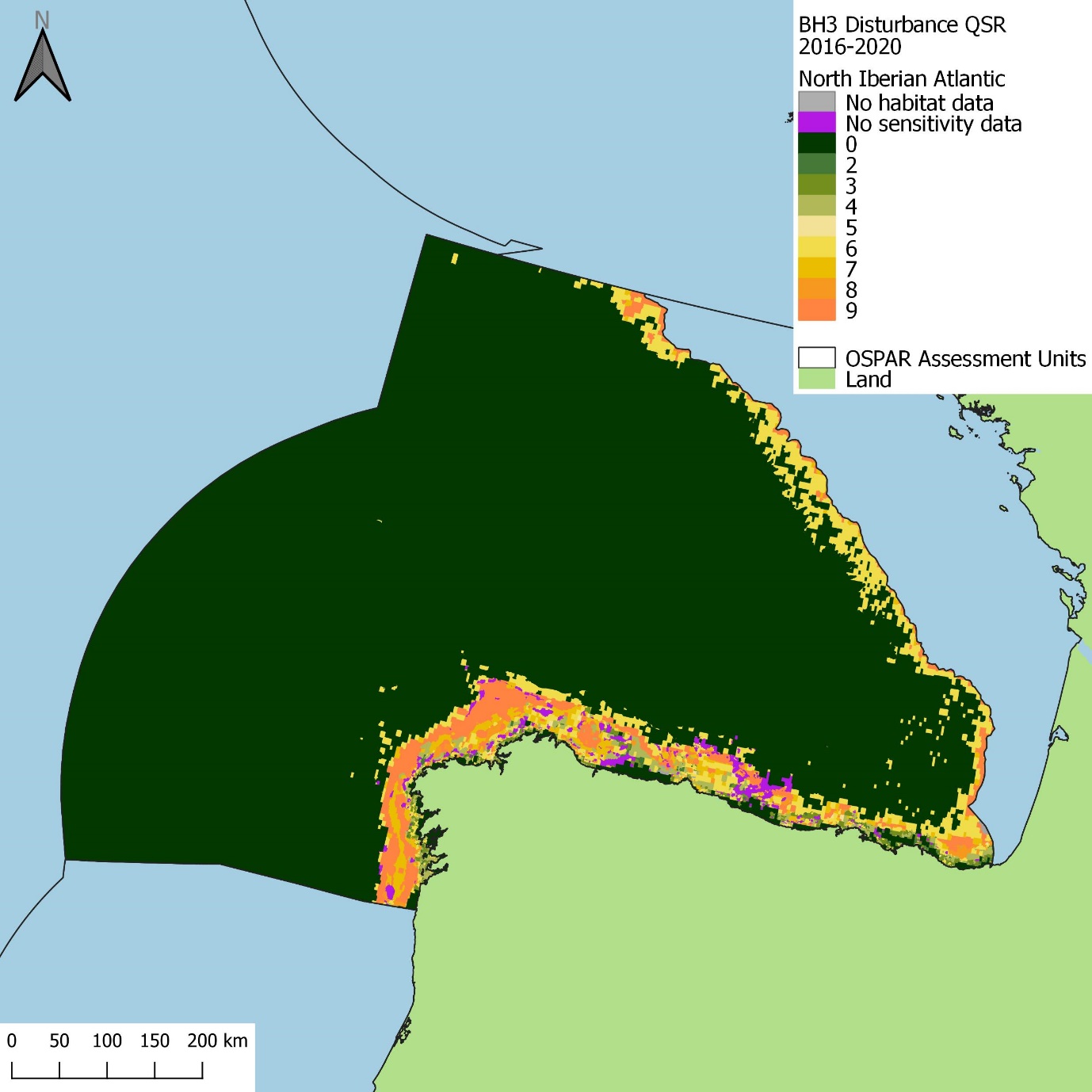
Figure be: Spatial distribution of aggregated disturbance within the North Iberian Atlantic assessment unit in the 2016 to 2020 assessment period
Assessment Unit Summary: South-Iberian Atlantic
In comparison to other assessment units, the South-Iberian Atlantic had the least percentage of area with disturbance (4%), largely due to a paucity of VMS data (Figure bh). ‘Moderate’ disturbance covered the largest proportion of the assessment unit (2%), followed by ‘Low’ (1%) and ‘High’ (<1%) (Figure bh). Disturbance was predominantly located along the margins of the continental shelf, with the highest disturbance located towards the north of the assessment unit (Figure bf). ‘Zero’ disturbance occurred in 95% of the South-Iberian Atlantic, due to VMS data paucity in deeper wates beyond the continental shelf edge and in coastal areas (Figure bf and Figure bh). Habitats with the highest proportions of area under ‘High’ disturbance were Upper bathyal sediment, followed by Offshore circalittoral mud (Figure bj).

Figure bf: Spatial distribution of aggregated disturbance within the South Iberian Atlantic assessment unit in the 2016 to 2020 assessment period
Assessment Unit Summary: Gulf of Cadiz
Approximately 72% of the Gulf of Cadiz had disturbance, with ‘High’ disturbance covering 32% of the assessment unit area, followed by both ‘Moderate’ and ‘Low’ at 20%, respectively (Figure bh). The highest disturbance was distributed in the north-west of the assessment unit, towards the central areas and parallel to the coastline. Additionally, 27% of the Gulf of Cadiz had ‘Zero’ disturbance, due to VMS data paucity, located towards the south-west of the assessment unit and the Strait of Gibraltar (Figure bg and Figure bh). Habitats with the greatest proportions of area under ‘High’ disturbance in the Gulf of Cadiz included Offshore circalittoral mud, Circalittoral mixed sediment and Circalittoral mud (Figure bj).
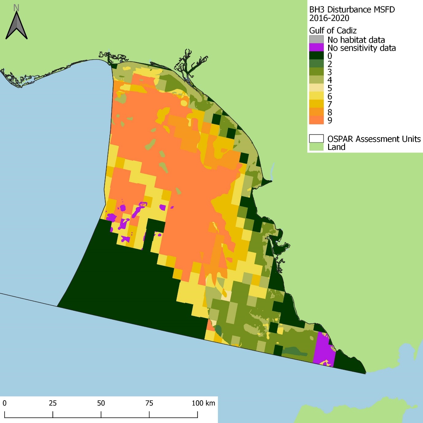
Figure bg: Spatial distribution of aggregated disturbance within the Gulf of Cadiz assessment unit in the 2016 to 2020 assessment period
Percentage of assessment unit area in each disturbance group
As observed in the 2009 to 2020 assessment period, the proportion of area in each disturbance group varied across assessment units (Figure bh). The greatest percentage of ‘High’ and ‘Moderate’ disturbance (67%) was in the Gulf of Biscay (‘High’ 21% and ‘Moderate’ 46%), followed closely by 58% in the Southern North Sea (‘High’ 13% and ‘Moderate’ 45%), 55% in the Central North Sea (‘High’ 21% and ‘Moderate 34%’), 52% in the Gulf of Cadiz (‘High’ 32% and ‘Moderate’ 20%), and 42% in the Southern Celtic Sea (‘High’ 14% and ‘Moderate’ 28%) (Figure bh). When disturbance groups were analysed individually, the greatest percentage of ‘High’ disturbance remained in the Gulf of Cadiz (32%) (Figure bh) and was predominantly distributed in the northwest of the assessment unit (Figure bg). Conversely the Channel had the greatest percentage of area with ‘Low’ disturbance, which still covered close to two thirds (64%) of the assessment unit, predominantly in western and central areas (Figure ay and Figure bh).
Despite the large area of ‘Low’ disturbance in the Channel, there were greater percentages of pressure categories 4 and 5 than were observed in the Gulf of Cadiz (Figure w). Therefore, the differences in disturbance between the two locations were the direct result of more sensitive habitats coinciding with higher intensities of pressure. For example, 100% of Offshore circalittoral mud had a surface / subsurface sensitivity score of 4 (Figure j and Figure k) in the Gulf of Cadiz. Although Offshore circalittoral mud only accounted for 11% of the total assessment unit area (Figure f), it coincided with very high surface pressure (5) (Figure v, Figure w and Figure aa, Figure l), and therefore was a key driver in the observed ‘High’ levels of disturbance (Figure bh). In contrast, equivalent levels of pressure in the Channel coincided with less sensitive habitats. Therefore, as observed in the 2009 to 2020 assessment period, pressure occurring over habitats with sensitivities of 4 or 5 was a greater contributor to higher levels of disturbance, than pressure intensity alone.
The greatest percentage of area with ‘Zero’ disturbance was observed in the South-Iberian and North-Iberian Atlantic (95% and 89% respectively; Figure bh), predominantly in offshore waters off the coast of Spain and Portugal. The assessment units with the least percentage of area with ‘Zero’ disturbance were the Southern North Sea, the Channel, and the Gulf of Biscay (all 8% or less; Figure bh). Notably the proportion of area with ‘Zero’ disturbance in the Gulf of Biscay was unchanged from the longer 2009 to 2020 assessment period (3%), despite the area of ‘Zero’ disturbance increasing for all other assessments units during the 2016 to 2020 assessment period. As ‘Zero’ disturbance demonstrated areas where no VMS data was reported throughout the assessment period, the widespread increase in ‘Zero’ disturbance within assessment units was likely driven by the 2016 to 2020 assessment period consisting of fewer years.
As highlighted in the 2009 to 2020 assessment period, it was not possible to distinguish whether areas without VMS were always true representations of ‘Zero’ disturbance. For example, ‘Zero’ disturbance was recorded in assessment units where data were not reported for certain fleets (although, these fleets were likely to be active), therefore, data interpretations in these locations should be treated with caution and caveated accordingly. However, where it was likely that fishing did not occur, such as waters deeper than 800 m (where bottom contact fishing is banned; (Deep-Sea Access Restriction EU 2016 / 2336), representations of ‘Zero’ disturbance had higher confidence (Figure af).
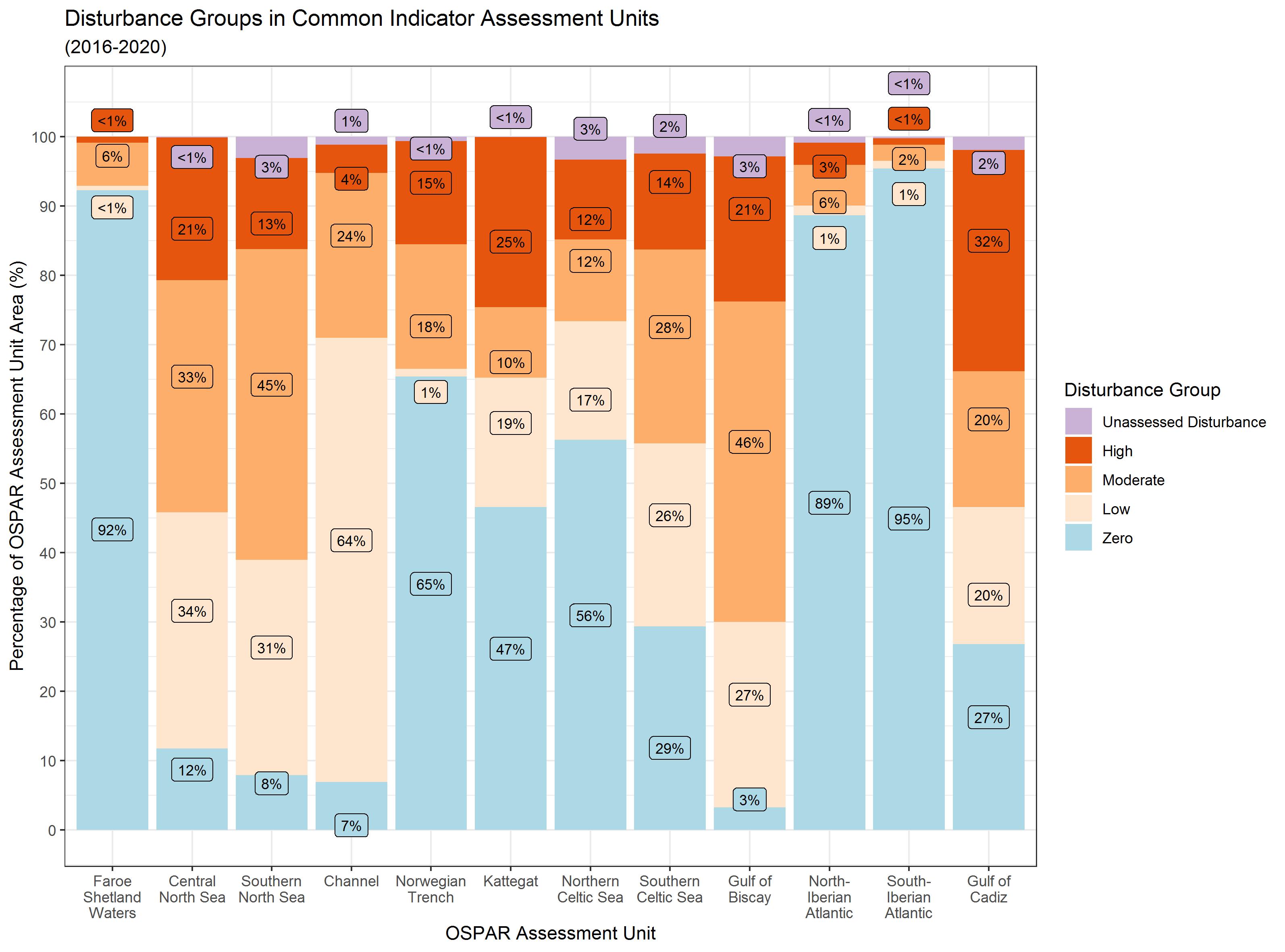
Figure bh: The percentage of OSPAR Common indicator assessment unit area under each of the following disturbance groups in the 2016 to 2020 assessment period: ‘Zero’ = disturbance category 0; ‘Low’ = disturbance categories 1-4; ‘Moderate’ = disturbance categories 5-7; ‘High’ = disturbance categories 8 and 9; ‘Unassessed Disturbance’ = area where fishing pressure was present but disturbance could not be assessed due to i) no habitat data, or ii) no sensitivity assessments for underlying habitat.
Disturbance within habitat types
When disturbance was analysed within the total area of each habitat across all assessment units (where BH3 is agreed as a Common Indictor), all 20 distinct BHTs had ‘High’ and / or ‘Moderate’ disturbance throughout the 2016 to 2020 assessment period (Figure bi). However, only three BHTs (Upper bathyal sediment, Offshore circalittoral sand, and Offshore circalittoral mud) had over 50% of their area in ‘Moderate’ and / or ‘High’ in the 2016 to 2020 assessment period. As observed in the 2009 to 2020 assessment period, Offshore circalittoral mud was the only habitat where over 50% of its area had ‘High’ disturbance (79%) (Figure bi). ‘Moderate’ disturbance was recorded in over 50% of the total area of Offshore circalittoral sand alone (64%). ‘Low’ disturbance was greatest in areas with Offshore circalittoral course sediment (87%), Offshore circalittoral mixed sediment (72%) and Infralittoral coarse sediment (61%) (Figure bi).
All 20 distinct BHTs had areas of ‘Zero’ disturbance, from 99% of the habitat area of Abyssal across all Common Indicator Assessment Units, to 6% in Offshore circalittoral mud. ‘Zero’ disturbance was recorded in over 50% of the area of seven BHTs: Abyssal (99%), Lower bathyal sediment (94%), Lower bathyal rock and biogenic reef (92%), Upper bathyal rock and biogenic reef (79%), Infralittoral mud (64%), Infralittoral rock and biogenic reef (60%), and Infralittoral mixed sediment (60%) (Figure bi).
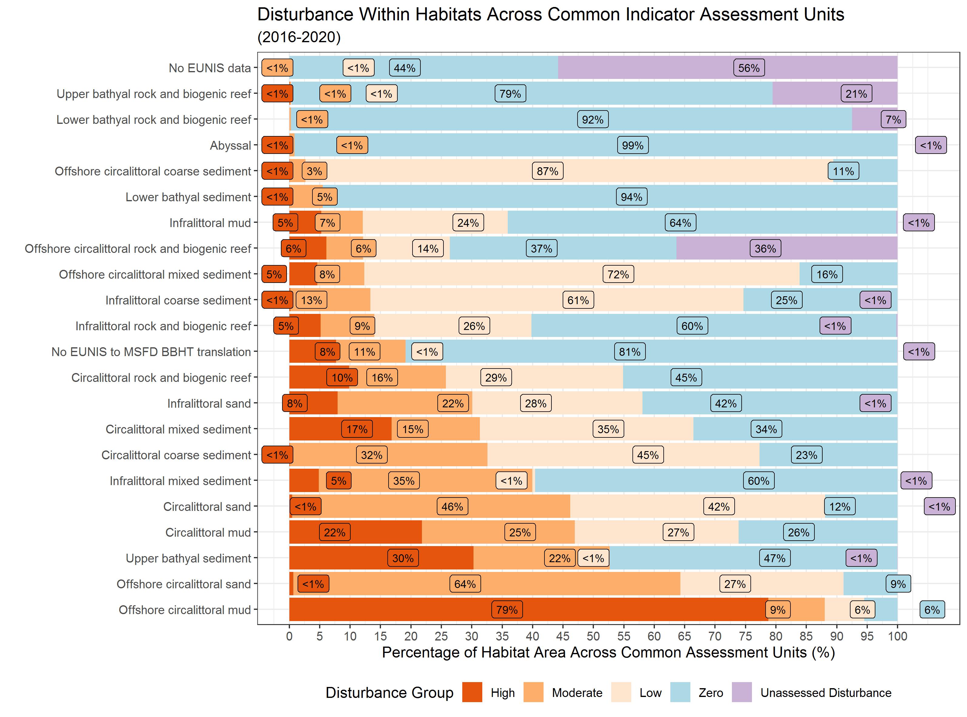
Figure bi: The percentage of each distinct BHT’s area across OSPAR Common Indicator Assessment Units under each of the following disturbance groups in the 2016 to 2020 assessment period: ‘High’ = disturbance categories 8 and 9; ‘Moderate’ = disturbance categories 5-7; ‘Low’ = disturbance categories 1-4; ‘Zero’ disturbance category 0; and ‘Unassessed Disturbance’ = area where fishing pressure was present but disturbance could not be assessed due to i) no habitat data, or ii) no sensitivity assessments for underlying habitat
Habitats with the greatest proportions of area without VMS data, and therefore ‘Zero’ disturbance, comprised Abyssal and Lower bathyal biological zones. The absence of VMS data can be attributed to reduced fishing in deep-sea areas due to trawl bans in depths greater than 800 m (Deep-Sea Access Restriction EU 2016 / 2336). However, it should be noted that disturbance values may have been underestimated in other habitats with potential gaps in VMS data, particularly in Infralittoral habitats due to aforementioned limitations such as a lack of data from vessels under 12 m in length. There were also notable nearshore areas without VMS data that can potentially be attributed to missing fleet data (e.g., Portuguese fleet in the South-Iberian Atlantic).
Habitat disturbance within assessment units
‘High’ and / or ‘Moderate’ disturbance was not observed in all distinct BHTs when analysing habitat disturbance in Common Indicator Assessment Units during the 2016 to 2020 assessment period. Of the 20 distinct BHTs, 14 (70% of BHTs), had ‘High’ and / or ‘Moderate’ disturbance in all Common Indicator Assessment Units in which they occurred (Table o and Figure bj). The 14 habitats ranged from the Infralittoral to the Abyssal zones, with particular prevalence of disturbance in the Circalittoral zone, where all habitats had ‘High’ and / or ‘Moderate’ disturbance in all Common Indicator Assessment Units they occurred in. ‘High’ and / or ‘Moderate’ disturbance was also observed in all assessment units where EUNIS to BHT translations were not possible; this was a result of translating from disturbance calculated at EUNIS Levels 2-6 to BHT. In addition, four BHTs (20%), ranging from Circalittoral to Bathyal zones, had ‘High’ disturbance in all assessment units they occurred in (Table o and Figure bj). Mud habitats were particularly affected as both Circalittoral and Offshore circalittoral mud had ‘High’ disturbance in all Common Indicator Assessment Units in which they occurred.
Furthermore, Offshore circalittoral mud had the greatest proportion of ‘High’ disturbance in eight of the 11 Common Indicator Assessment Units in the 2016 to 2020 assessment period (Figure bj); one fewer assessment unit than in the 2009 to 2020 assessment period. In the South-Iberian Atlantic and the Central North Sea, the greatest percentage of ‘High’ disturbance remained in Upper bathyal sediment. However, in the Southern North Sea the greatest percentage of ‘High’ disturbance occurred in areas where no EUNIS to BHT translation was possible.
The differences observed in habitats with the greatest proportions of ‘High’ disturbance in the South-Iberian Atlantic, Central North Sea, and Southern North Sea (when compared to other Common Indicator Assessment Units) were due to a variety of reasons. In the South-Iberian Atlantic, lower levels of disturbance were observed in Offshore circalittoral mud due to reduced surface pressure intensity and coverage within the habitat (Figure aa). In the Central North Sea and Southern North Sea, the percentage of ‘High’ disturbance in Offshore circalittoral mud aligned with other assessment units. However, a greater proportion of ‘High’ disturbance was observed in Upper bathyal sediment and areas with no EUNIS to BHT translation, respectively, due to a combination of increased pressure intensity and coverage (Figure aa). It should be noted that this was likely due to Upper bathyal sediment and areas with no EUNIS to BHT translation covering relatively small areas of the Central North Sea and Southern North Sea respectively (<1%) (Figure f).
Offshore circalittoral sand had the greatest percentage of habitat area with ‘Moderate’ disturbance in eight of 11 assessment units during the 2016 to 2020 assessment period (Figure bj); two assessment units fewer than during the 2009 to 2020 assessment period. In the Central North Sea and the Gulf of Cadiz, Infralittoral mixed sediment had the greatest percentages of ‘Moderate’ disturbance; in the South-Iberian Atlantic, Upper bathyal sediment had the greatest percentage of ‘Moderate’ disturbance (Figure bj). In the Central North Sea, pressure intensity and coverage over Offshore circalittoral sand were similar to other assessment units. However, there was very little difference between pressure coverage in Offshore circalittoral sand and Infralittoral mixed sediment (a more sensitive habitat), resulting in higher levels of ‘Moderate’ disturbance in Infralittoral mixed sediment. In the Gulf of Cadiz, surface pressure intensity in Offshore circalittoral sand was substantially lower than in other assessment units, resulting in an increase in the proportion of ‘Low’ rather than ‘Moderate’ disturbance within the habitat. In the South-Iberian Atlantic a combination of less pressure coverage and a greater proportion of low intensity surface pressure in Offshore circalittoral sand led to a reduction in the percentage of ‘Moderate’ disturbance in the habitat.
Table o: The presence of ‘High’ (disturbance categories 8 and 9) and ‘Moderate’ (disturbance categories 5-7) disturbance groups within habitats across OSPAR benthic assessment units the habitat occurs in, where BH3 is agreed as Common, in the 2016 to 2020 assessment period. Blue shading indicates the biological zone of the habitat; ticks indicate that the disturbance group was present across all assessment units the habitat occurred in; crosses indicate the disturbance group was not present in all assessment units that the habitat occurred in
| BHT | High and/or Moderate | High |
|---|---|---|
| Infralittoral rock and biogenic reef | ü | û |
| Infralittoral coarse sediment | û | û |
| Infralittoral mixed sediment | ü | û |
| Infralittoral sand | ü | û |
| Infralittoral mud | û | û |
| Circalittoral rock and biogenic reef | ü | û |
| Circalittoral coarse sediment | ü | û |
| Circalittoral mixed sediment | ü | ü |
| Circalittoral sand | ü | û |
| Circalittoral mud | ü | ü |
| Offshore circalittoral rock and biogenic reef | ü | û |
| Offshore circalittoral coarse sediment | û | û |
| Offshore circalittoral mixed sediment | û | û |
| Offshore circalittoral sand | ü | û |
| Offshore circalittoral mud | ü | ü |
| Upper bathyal rock and biogenic reef | û | û |
| Upper bathyal sediment | ü | ü |
| Lower bathyal rock and biogenic reef | û | û |
| Lower bathyal sediment | û | û |
| Abyssal | ü | û |
| No EUNIS to MSFD BBHT translation | ü | û |
| No EUNIS data | û | û |
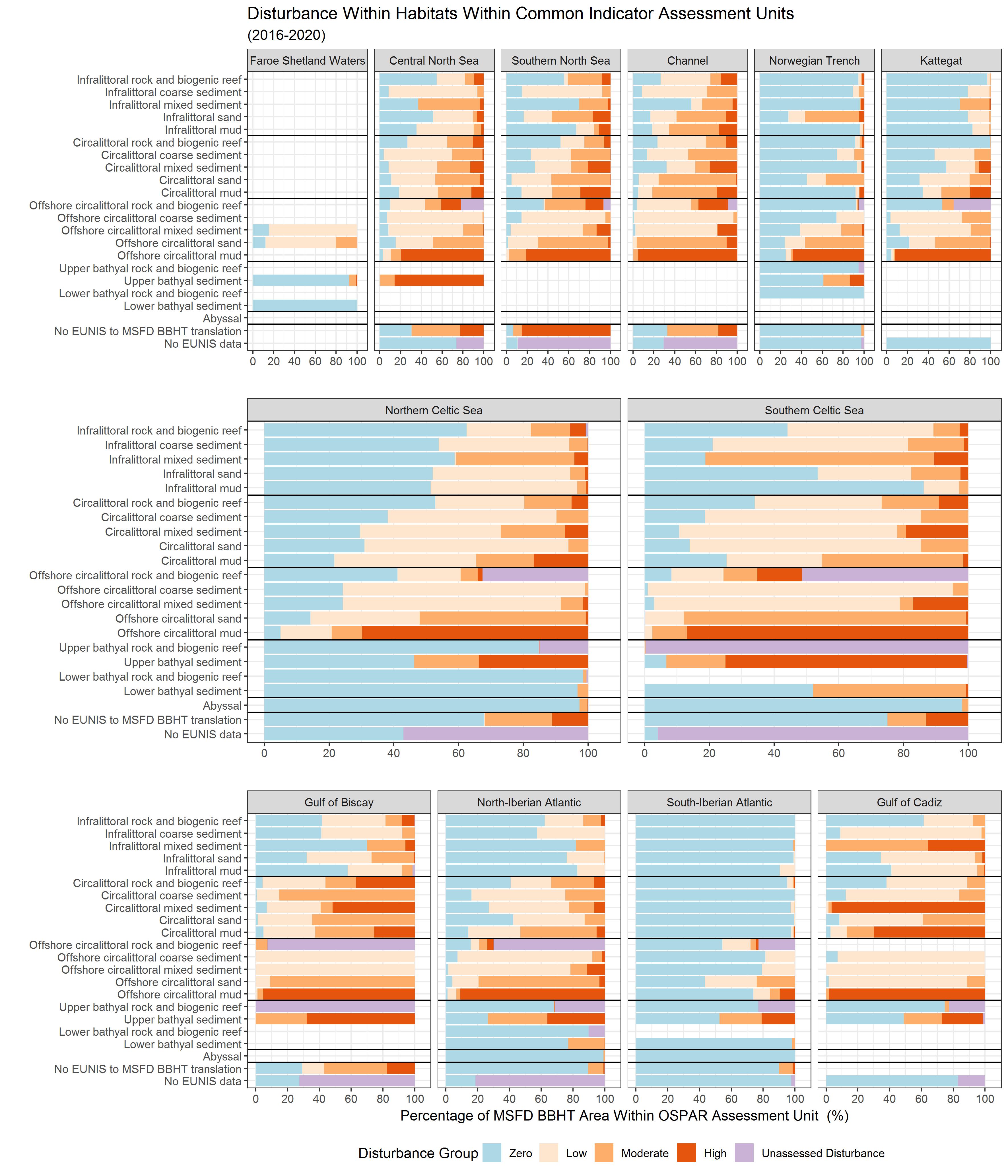
Figure bj: The percentage of BHT area in each OSPAR Common Indicator Assessment Unit under each of the following disturbance groups in the 2016 to 2020 assessment period: ‘Zero’ = disturbance category 0; ‘Low’ = disturbance categories 1-4; ‘Moderate’ = disturbance categories 5-7; ‘High’ = disturbance categories 8 and 9; ‘Unassessed Disturbance’ = area where fishing pressure was present but disturbance could not be assessed due to i) no habitat data, or ii) no sensitivity assessments for underlying habitat. Horizontal black lines represent the separation in biological zones
As observed in the 2009 to 2020 assessment period both Offshore circalittoral coarse sediment and Offshore circalittoral mixed sediment had large percentages of ‘Low’ disturbance in Common Indicator Assessment Units during the 2016 to 2020 assessment period (Figure bj). Offshore circalittoral coarse sediment had the greatest percentage of ‘Low’ disturbance in seven of the 11 assessment units (Central North Sea, Channel, Southern North Sea, Kattegat, Northern Celtic Sea, Southern Celtic Sea, and North-Iberian Atlantic); one fewer than during the 2009 to 2002 assessment period. Offshore circalittoral mixed sediment had the greatest percentage of ‘Low’ disturbance in two of the 11 assessment units (Norwegian Trench and Gulf of Cadiz). In the Gulf of Biscay both Offshore circalittoral coarse sediment and Offshore circalittoral mixed sediment had 100% of their area in ‘Low’ disturbance. In contrast to the 2009 to 2020 assessment period, the South-Iberian Atlantic was the only assessment unit where the greatest proportion of ‘Low’ disturbance was in Offshore circalittoral sand, due to a substantial increase in low intensity surface pressure within the habitat, as previously discussed.
Infralittoral mixed sediment, Abyssal, and Infralittoral rock and biogenic reef habitats had large percentages of ‘Zero’ disturbance within Common Indicator Assessment Units (Figure bj). Infralittoral mixed sediment had the greatest percentage of area with ‘Zero’ disturbance in four of the 11 Common Indicator Assessment Units (Channel, Gulf of Biscay, Norwegian Trench, and Southern North Sea). Infralittoral rock and biogenic reef had the greatest percentage of area with ‘Zero’ disturbance in two of the 11 Common Indicator Assessment Units (Central North Sea and South-Iberian Atlantic). Abyssal also had the greatest percentage of area with ‘Zero’ disturbance in another two of the 11 Common Indicator Assessment Units (North-Iberian Atlantic and Southern Celtic Sea). The BHTs with the largest percentage of area with ‘Zero’ disturbance all differed in the remaining three Common Indicator Assessment Units, but ranged from Lower bathyal to Circalittoral biological zones.
In the Gulf of Cadiz, where the greatest percentage of ‘High’ disturbance was observed, ‘High’ disturbance covered more than 90% of the area of Circalittoral mixed sediment and Offshore circalittoral mud, and over 50% of Circalittoral mud during the 2016 to 2020 assessment period (Figure bj). These observations in the Gulf of Cadiz aligned with findings from the 2009 to 2020 assessment period. However, as stated in the 2009 to 2020 assessment, Circalittoral mixed sediment covered a relatively small area of the Gulf of Cadiz (1%), while Circalittoral mud and Offshore circalittoral mud both covered more than 10% of the assessment unit, respectively (Figure f). Therefore, Circalittoral mud and Offshore circalittoral mud made greater contributions to the large percentage of ‘High’ disturbance in the Gulf of Cadiz.
In the Channel, where the greatest proportion of ‘Low’ disturbance was observed, ‘Low’ disturbance covered more than 90% Offshore circalittoral coarse sediment during the 2016 to 2020 assessment period (Figure bj). These observations in the Channel also aligned with findings from the 2009 to 2020 assessment period. In addition, over 50% of Offshore circalittoral rock and biogenic reef, Offshore circalittoral mixed sediment and Infralittoral coarse sediment in the Channel remained under ‘Low’ disturbance (Figure bj). Offshore circalittoral mud remained the only habitat in the Channel with the majority of its area under ‘High’ disturbance (over 90%). As stated in the 2009 to 2020 assessment, Offshore circalittoral mud had a very low extent of coverage in the Channel (less than 1%) (Figure f), meaning that it had little effect on the overall disturbance recorded in the assessment unit.
Disturbance trends over time
Annual disturbance varied throughout the time series, although, no clear trends were detected (Figure bk). However, annual variations in disturbance did indicate that the large proportion of ‘High’ disturbance in the aggregated Gulf of Cadiz assessment (Figure bh) may have been driven by peaks in disturbance observed in 2018 and 2020 alone (Figure bk). In contrast, between 2009 and 2017, the majority of disturbance in the Gulf of Cadiz was ‘Low’ (Figure bk).
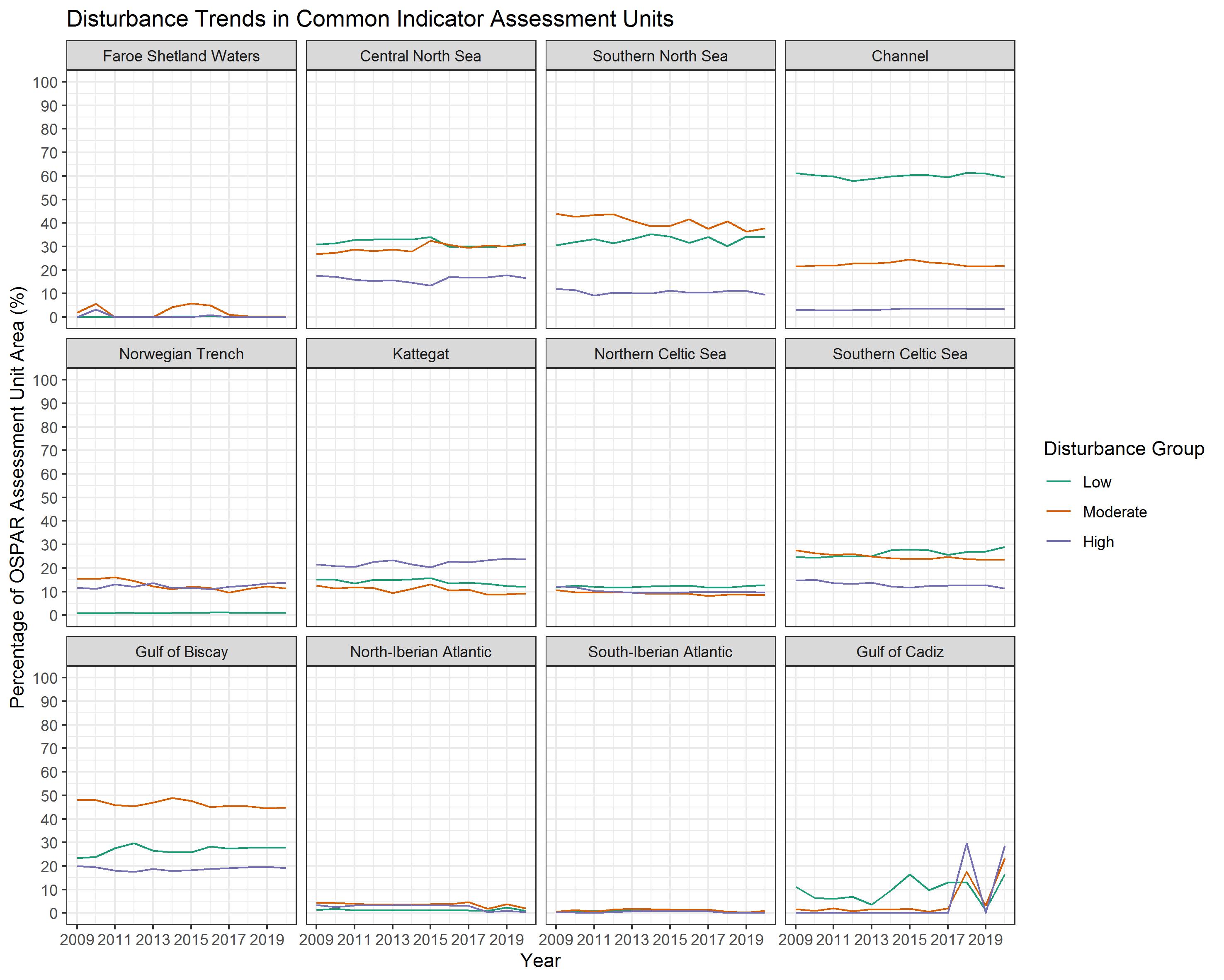
Figure bk: The annual percentage of OSPAR Common Indicator Assessment Unit areas under the disturbance groups: ‘Low’ (disturbance categories 1-4), ‘Moderate’ (disturbance categories 5-7) and ‘High’ (disturbance categories 8 and 9) between the years 2009 to 2020.
The Kattegat was the only assessment unit where the majority of disturbance was consistently ‘High’, which also showed a slight increase over time (Figure bk). Conversely, the Channel was the only assessment unit where the greatest proportion of area had consistently ‘Low’ disturbance throughout the time series (Figure bk), which aligned with overall aggregated disturbance results (Figure bh and Figure bk).
Overall results for Region V (Candidate Indicator Assessment)
2009-2020:
In total, 11% of the area of the Atlantic Projection assessment unit had disturbance (Figure bm). ‘Moderate’ disturbance covered the largest proportion of the assessment unit (9%), followed by ‘High’ and ‘Low’ (2% and <1% respectively) (Figure bm). The highest disturbance within the assessment unit was found around Hatton Bank and Rockall Bank (Figure bl). Additionally, ‘Zero’ disturbance occurred throughout 89% of the assessment unit due to areas without reported SAR values. However, most of the assessment unit consisted of deep-sea habitats (Figure c), which were not likely to be suitable for bottom contact fishing.
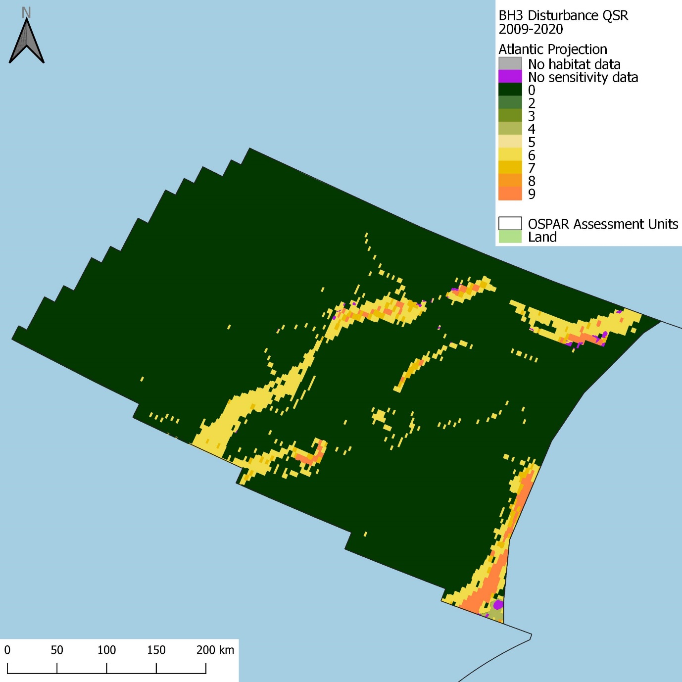
Figure bl: Spatial distribution of aggregated disturbance within the Atlantic Projection Candidate Indicator Assessment Unit in the 2009 to 2020 assessment period
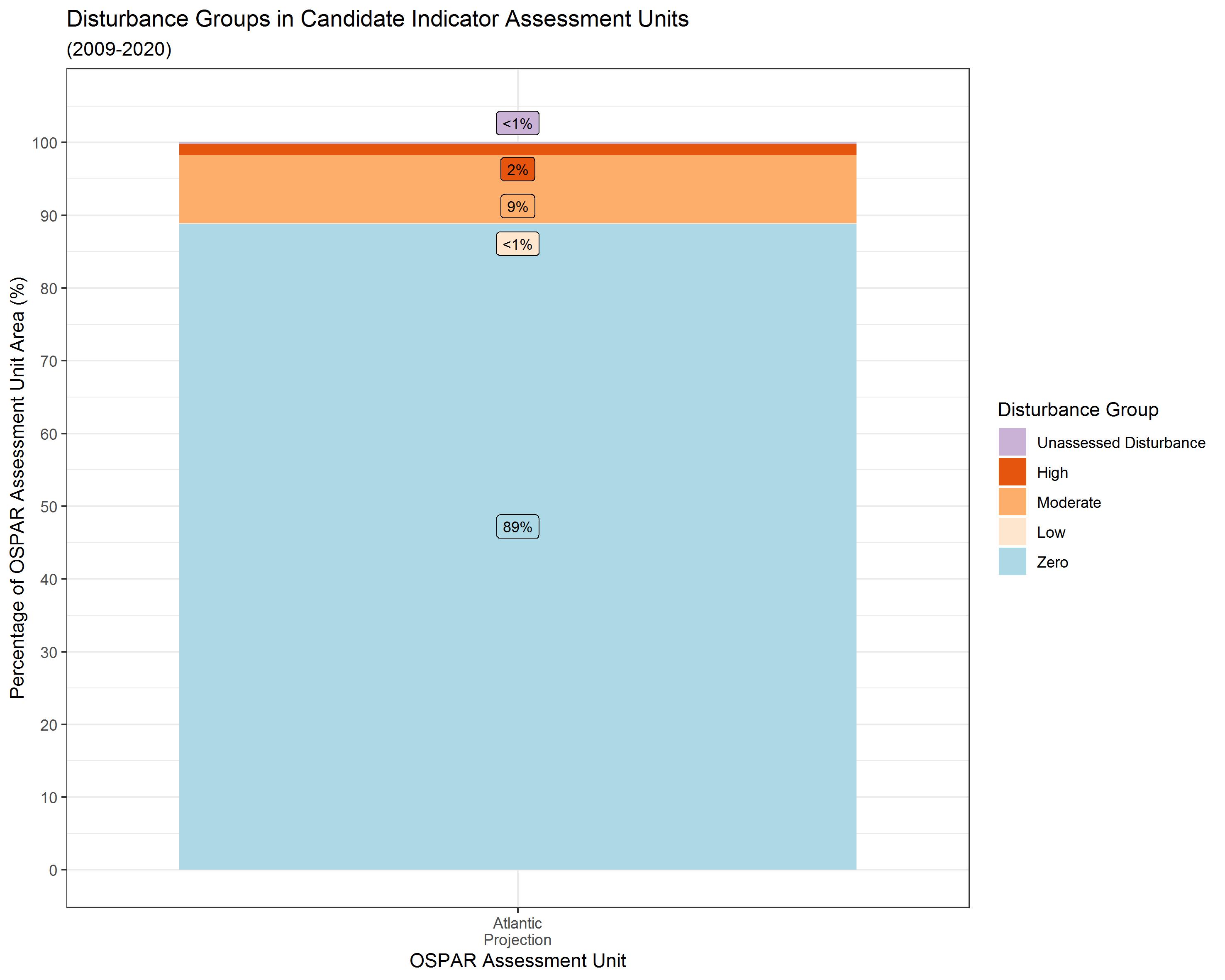
Figure bm: The percentage of OSPAR Candidate Indicator Assessment Unit area under each of the following disturbance groups in the 2009 to 2020 assessment period: ‘Zero’ = disturbance category 0; ‘Low’ = disturbance categories 1-4; ‘Moderate’ = disturbance categories 5-7; ‘High’ = disturbance categories 8 and 9; ‘Unassessed Disturbance’ = area where fishing pressure was present but disturbance could not be assessed due to i) no habitat data, or ii) no sensitivity assessments for underlying habitat. Horizontal black lines represent the separation in biological zones
2016-2020
In total, ~5% of the area of the Atlantic Projection assessment unit had disturbance (Figure bm). ‘Moderate’ disturbance covered the largest proportion of the assessment unit (5%), followed by ‘High’ and ‘Low’ (both <1%) (Figure bm). The highest disturbance within the assessment unit was found around Hatton Bank and Rockall Bank (Figure bn). Additionally, ‘Zero’ disturbance occurred throughout 89% of the assessment unit due to areas without reported SAR values. However, most of the assessment unit consisted of deep-sea habitats (Figure c) that were likely not to be suitable for bottom-contact fishing.
Figure bn: Spatial distribution of aggregated disturbance within the Atlantic Projection Candidate Indicator Assessment Unit in the 2016 to 2020 assessment period
Figure bo: The percentage of OSPAR Candidate Indicator Assessment Unit area under each of the following disturbance groups in the 2016 to 2020 assessment period: ‘Zero’ = disturbance category 0; ‘Low’ = disturbance categories 1-4; ‘Moderate’ = disturbance categories 5-7; ‘High’ = disturbance categories 8 and 9; ‘Unassessed Disturbance’ = area where fishing pressure was present but disturbance could not be assessed due to i) no habitat data, or ii) no sensitivity assessments for underlying habitat. Horizontal black lines represent the separation in biological zones
Assessments of OSPAR Threatened and / or Declining Habitats: 2009 to 2020
Figure bp: OSPAR Threatened and / or Declining Habitats polygons (EMODnet, 2020)
Figure bq: Spatial distribution of aggregated disturbance for OSPAR Threated and / or Declining Habitats in the 2009 to 2020 assessment period
OSPAR Threated and / or Declining Habitats were reported in nine of the Common Indicator Assessment Units (Figure bp). None of the assessed habitats were reported in the Gulf of Biscay, South-Iberian Atlantic, or the Candidate Indicator Assessment Unit (Atlantic Projection). The greatest areas of habitats were reported in the Northern Celtic Sea and Southern North Sea (Figure bt). Please note, an assessment of Zostera could not be completed due to errors in available habitat data, preventing accurate analyses in GIS; these data will be considered for analyses in future assessments.
All assessment units with reported OSPAR Threated and / or Declining Habitats had a proportion of at least one habitat with disturbance in the QSR assessment period (Figure bq and Figure bs). The largest areas of ‘High’ disturbance were in the Northern Celtic Sea, Central North Sea, and Southern North Sea.
Disturbance results were reported in all areas where surface or subsurface pressure intersected with habitat polygons. However, it should be noted that pressure data were solely available at a c-square resolution (pressure assumed to be homogeneous within a given c-square). Therefore, in some instances of shallow / intertidal habitats (e.g., Littoral chalk communities), fishing activity potentially occurred adjacent to the assessed habitat within the same c-square.
Littoral chalk communities
At the time of assessment, Littoral chalk communities were reported in the Central and Southern North Sea, the Northern and Southern Celtic Sea, and the Channel. In the 2009 to 2020 assessment period, physical disturbance occurred in 50% of the total area of Littoral chalk communities across all Common Indicator Assessment Units (41,57 km2: Figure br and Figure bt). ‘High’ disturbance affected 30% of the total habitat area, ‘Low’ disturbance affected 20%, and ‘Moderate’ disturbance was not observed (Figure br). Most ‘High’ disturbance in Littoral chalk communities was confined to the Channel, where the greatest extent of the habitat was observed (35,86 km2) (Figure bs and Figure bt). A small percentage of area of Littoral chalk communities had ‘High’ disturbance in the Southern North Sea, but most of the assessed disturbance was ‘Low’ in this assessment unit, 13% of the 5,56 km2 habitat area (Figure bs). There was less than 0,2 km2 total habitat area In the Central North Sea, Northern and Southern Celtic Sea together, where only ‘Low’ disturbance occurred (Figure bs).
Intertidal mudflats
At the time of assessment, Intertidal mudflats were reported in the Central and Southern North Sea, the Northern and Southern Celtic Sea, the Channel, the Norwegian Trench, and the Kattegat. In the 2009 to 2020 assessment period, physical disturbance occurred in 70% of the total area of Intertidal mudflats across all Common Indicator Assessment Units where the feature was present (6 407,46 km2) and both pressure and sensitivity data were available (Figure br and Figure bt). Both ‘Moderate’ and ‘Low’ disturbance occurred 35% of the total habitat area (Figure br). Most of the ‘Moderate’ and ‘Low’ disturbance in Intertidal mudflats occurred in the Southern North Sea where the greatest extent of the habitat was observed (5 565,39 km2), 41% and 40% of habitat area respectively (Figure bs and Figure bt). Areas of ‘Low’ and ‘Moderate’ disturbance in Intertidal mudflats was less than 10% of habitat area in the Channel, the Norwegian Trench, the Kattegat, and the Northern and Southern Celtic Sea (Figure bs).
Intertidal Mytilus edulis beds on mixed and sandy sediments
At the time of assessment, Intertidal Mytilus edulis beds on mixed and sandy sediments were reported in the Central and Southern North Sea, the Northern and Southern Celtic Sea, the Channel, the Norwegian Trench and the Kattegat, with a total area of 135,07 km2 (Figure bt). Disturbance occurred in 70% of the total area of Intertidal Mytilus edulis beds on mixed and sandy sediments across Common Indicator Assessment Units in the 2009 to 2020 assessment period (Figure br). ‘Low’ disturbance occurred in a greater proportion of total habitat area (48%) than ‘Moderate’ disturbance (22%; Figure br). The largest proportion of ‘Moderate’ disturbance in Intertidal Mytilus edulis beds on mixed and sandy sediments occurred in the Channel, where 45% and 49% of the habitat area had ‘Moderate’ and ‘Low’ disturbance respectively (Figure bs). ‘Moderate’ disturbance was also present in the Southern North Sea (24% of habitat extent) and a small amount in the Norwegian Trench (1%; Figure bs). With the exception of the Kattegat, ‘Low’ disturbance occurred in all assessment units where Intertidal Mytilus edulis beds on mixed and sandy sediments were found. The Southern North Sea had the greatest extent of habitat area (84,11 km2) and also the largest proportion of ‘Low’ disturbance (60%; Figure bs and Figure bt).
Ostrea edulis beds
At the time of assessment, the area Ostrea edulis beds reported was minimal (0,68 km2) and restricted to the Southern North Sea and the Norwegian Trench (Figure bt). Fishing activity in the 2009 to 2020 assessment period did not overlap the reported habitat area and disturbance in Ostrea edulis beds in both assessment units was ‘Zero’ (Figure bs).
Modiolus modiolus horse mussel beds
At the time of assessment, Modiolus modiolus horse mussel beds were reported in the Central North Sea and the Northern Celtic Sea. In the 2009 to 2020 assessment period, physical disturbance occurred in less than 21% of the total area of Modiolus modiolus horse mussel beds across all Common Indicator Assessment Units where the feature was present (49,99 km2 total area; Figure br and Figure bt). Disturbance was predominantly ‘Low’ (21%), followed by ‘Moderate’ (<1%) and ‘High’ (<1%), (Figure br). ‘High’ disturbance only occurred in Modiolus modiolus horse mussel beds in the Central North Sea and in a small area (<1% of habitat within the assessment unit; Figure bs). ‘Moderate’ disturbance only occurred in the Northern Celtic Sea, with 2% of the habitat within the assessment unit affected (Figure bs). ‘Low’ disturbance in Modiolus modiolus habitat was present in both the Central North Sea and Northern Celtic Sea, 21% and 20% of habitat area, respectively (Figure bs).
Maerl beds
At the time of assessment, Maerl beds were reported in the Central North Sea, the Northern and Southern Celtic Sea, and the Channel. In the 2009 to 2020 assessment period, physical disturbance occurred in 45% of the total area of Maerl beds across all Common Indicator Assessment Units where the feature was present (154,67 km2; Figure br and Figure bt). Disturbance across assessment units comprised of ‘Moderate’, 38% of total habitat area, and ‘High’, 7% of total habitat area (Figure br). ‘High’ disturbance in Maerl beds was only found in the Northern Celtic Sea, 8% of the 125,28 km2 habitat area (Figure bs); this was also the assessment unit with the greatest extent of Maerl beds (Figure b). The greatest proportion of disturbance in Maerl bed habitat within an assessment unit occurred in the Southern Celtic Sea, with 81% of the 22,01 km2 in ‘Moderate’ disturbance (Figure bs and Figure bt).
Sabellaria spinulosa reefs
At the time of assessment, Sabellaria spinulosa reefs were reported in the Central and Southern North Sea, the Northern and Southern Celtic Sea and the Channel. In the 2009 to 2020 assessment period, physical disturbance occurred in 74% of the total area of Sabellaria spinulosa reefs across all Common Indicator Assessment Units where the feature was present (840,19 km2; Figure br and Figure bt). Of the total habitat area of Sabellaria spinulosa reefs, over half (57%) had ‘Low’ disturbance, followed by ‘High’ (11%) and ‘Moderate’ (6%; Figure br). Within assessment units, ‘High’ disturbance in Sabellaria spinulosa reefs only occurred in the Southern North Sea (13% of habitat area) (Figure bs), which was also the assessment unit with the largest extent of habitat (690,41 km2; Figure bt). The proportion of habitat under ‘Moderate’ disturbance was greatest in the Southern Celtic Sea, 38% of the 67,47 km2 habitat area. All of the reported Sabellaria spinulosa reef habitat in the Northern Celtic Sea (20,58 km2) had ‘Low’ disturbance (Figure bs).
Sea-pen and burrowing megafauna communities
At the time of assessment, Sea-pen and burrowing megafauna communities were reported in the Central and Southern North Sea, the Northern and Southern Celtic Sea, and the Gulf of Cadiz. In the 2009 to 2020 assessment period, physical disturbance occurred in 98% of the total area of Sea-pen and burrowing megafauna communities across all Common Indicator Assessment Units where the feature was present (12 863,74 km2; Figure br and Figure bt). Over 90% of the assessed area of the feature had ‘High’ disturbance, followed by ‘Low’ at 6% and ‘Moderate’ at 2% across assessment units where it was present (Figure br). In all assessment units where Sea-pen and burrowing megafauna communities were found, ‘High’ disturbance was the predominant disturbance category for the habitat and was recorded as over 95% of habitat extent in the Central and Southern North Sea, and Southern Celtic Sea (Figure bs). In the Southern North Sea, Southern Celtic Sea, and Gulf of Cadiz all of the reported habitat area experienced disturbance in the 2009 to 2020 assessment period. Only 3% and less than 1% of the habitat area in the Northern Celtic Sea and Central North Sea respectively had ‘Zero’ disturbance (Figure bs).
Deep-sea sponge aggregations
At the time of assessment, Deep-sea sponge aggregations were reported in the North-Iberian Atlantic and the Gulf of Cadiz. In the 2009 to 2020 assessment period, physical disturbance occurred in 43% of the total area of Deep-sea sponge aggregations in all Common Indicator Assessment Units where the feature was present (491,9 km2; Figure br and Figure bt). When considering the total habitat area, 40% had ‘Moderate’ disturbance and 3% had ‘High’ disturbance (Figure br). The greatest proportion of disturbance of Deep-sea sponge aggregations was observed in the Gulf of Cadiz, 5% area had ‘High’ and 58% had ‘Moderate’ disturbance (Figure bs). However, the total habitat area was smaller in the Gulf of Cadiz (49,82 km2) than the North-Iberian Atlantic (442,08 km2; Figure bt), which had 38% and 3% area with ‘Moderate’ and ‘High’ disturbance respectively (Figure bs).
Coral gardens
At the time of assessment, Coral gardens were reported in the Northern Celtic Sea, the North-Iberian Atlantic and the Gulf of Cadiz. In the 2009 to 2020 assessment period, physical disturbance occurred in less than 1% of the total area of Coral gardens across all Common Indicator Assessment Units where the feature was present (970,77 km2; Figure br and Figure bt). ‘Moderate’ disturbance covered a large proportion of habitat area in the Northern Celtic Sea (39%), although there was only a minimal area of Coral garden habitat reported in the assessment unit (2,5 km2; Figure bs and Figure bt). ‘High’ disturbance as a proportion of habitat area was greatest in the Gulf of Cadiz (4%), which had 21,29 km2 habitat area reported. The greatest extent of Coral garden habitat was reported in the North-Iberian Atlantic (946,99 km2) with the total area having ‘Zero’ disturbance (Figure bs and Figure bt).
Lophelia pertusa reefs
At the time of assessment, Lophelia pertusa reefs were reported in the Northern and Southern Celtic Sea, the North-Iberian Atlantic and the Gulf of Cadiz. In the 2009 to 2020 assessment period, physical disturbance occurred in 14% of the total area of Lophelia pertusa reefs across all Common Indicator Assessment Units where the feature was present (197,98 km2; Figure br and Figure bt). When considering the total area of Lophelia pertusa reefs, ‘Moderate’ disturbance contributed to the greatest proportion of disturbance (12% of habitat area), followed by ‘High’ (2%; Figure br). The greatest proportion of Lophelia pertusa reefs that had ‘High’ disturbance (2% of habitat extent) was observed in the North-Iberian Atlantic (Figure bs); the North-Iberian Atlantic also had the largest extent of Lophelia pertusa reefs (170,2 km2; Figure bt). Small areas of Lophelia pertusa reefs in the Southern Celtic Sea and Gulf of Cadiz (0.,17 km2 and 0,38 km2 respectively) had ‘Moderate’ disturbance (Figure bs and Figure bt).
Carbonate mounds
At the time of assessment, Carbonate mounds were reported in the Northern and Southern Celtic Sea, and the Gulf of Cadiz. In the 2009 to 2020 assessment period, physical disturbance occurred in 59% of the total area of Carbonate mounds across all Common Indicator Assessment Units (250,39 km2; Figure br and Figure bt). When considering the total area of Carbonate mounds, disturbance was predominantly ‘Moderate’ (52%), followed by ‘High’ (7%; Figure br). The greatest proportion of disturbance within an assessment unit occurred in the Gulf of Cadiz, where the 2,37 km2 of the habitat had ‘High’ or ‘Moderate’ disturbance (54% and 46% respectively; Figure bs and Figure bt). Proportions of ‘Moderate’ disturbance within the Northern and Southern Celtic Sea were also high (41% and 65% respectively), where the Northern Celtic Sea also had 10% of the total 131,82 km2 habitat area in ‘High’ disturbance.
Seamounts
At the time of assessment, Seamounts were reported in the Northern Celtic Sea only. In the 2009 to 2020 assessment period, physical disturbance occurred in over half (53%) of the total area of Seamounts (8 022,8 km2) in the Northern Celtic Sea. The proportion of habitat extent that had ‘Moderate’ disturbance was greatest at 49%, followed by ‘High’ with 4% (Figure br and Figure bt).
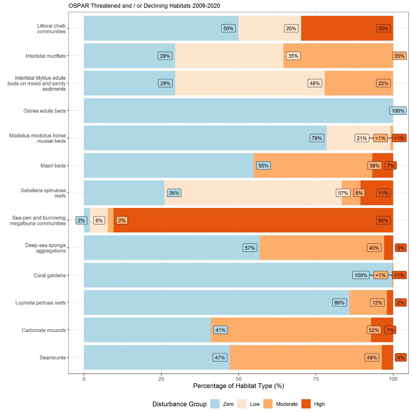
Figure br: The percentage of each OSPAR Threated and / or Declining Habitat’s area (across OSPAR benthic assessment units where BH3 is agreed as a Common Indicator) under each of the following disturbance groups in the 2009 to 2020 assessment period: ‘Zero’ = disturbance category 0; ‘Low’ = disturbance categories 1-4; ‘Moderate’ = disturbance categories 5-7; ‘High’ = disturbance categories 8 and 9
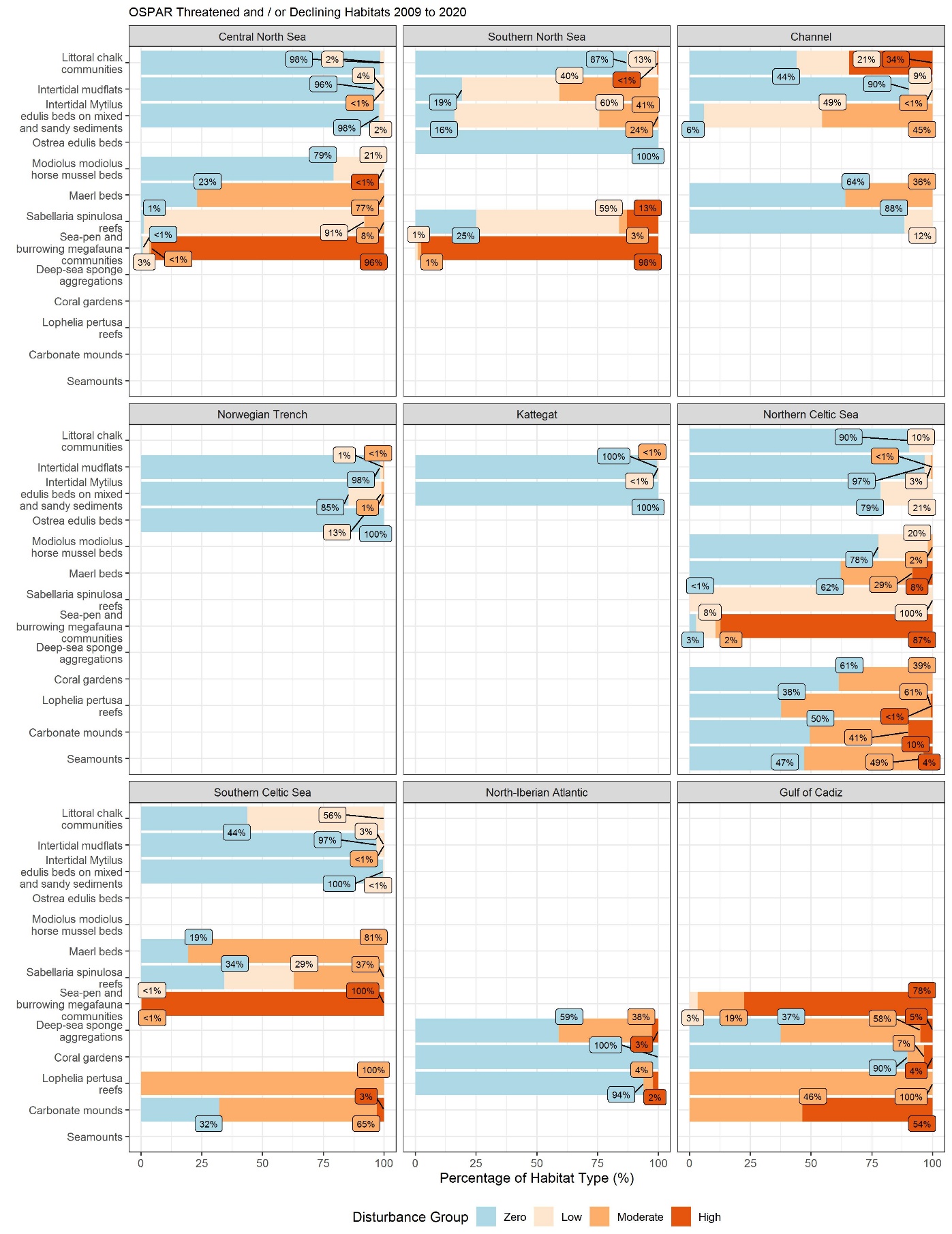
Figure bs: The percentage of each OSPAR Threated and / or Declining Habitat’s area (within OSPAR benthic assessment units where BH3 is agreed as a Common Indicator) under each of the following disturbance groups in the 2009 to 2020 assessment period: ‘Zero’ = disturbance category 0; ‘Low’ = disturbance categories 1-4; ‘Moderate’ = disturbance categories 5-7; ‘High’ = disturbance categories 8 and 9
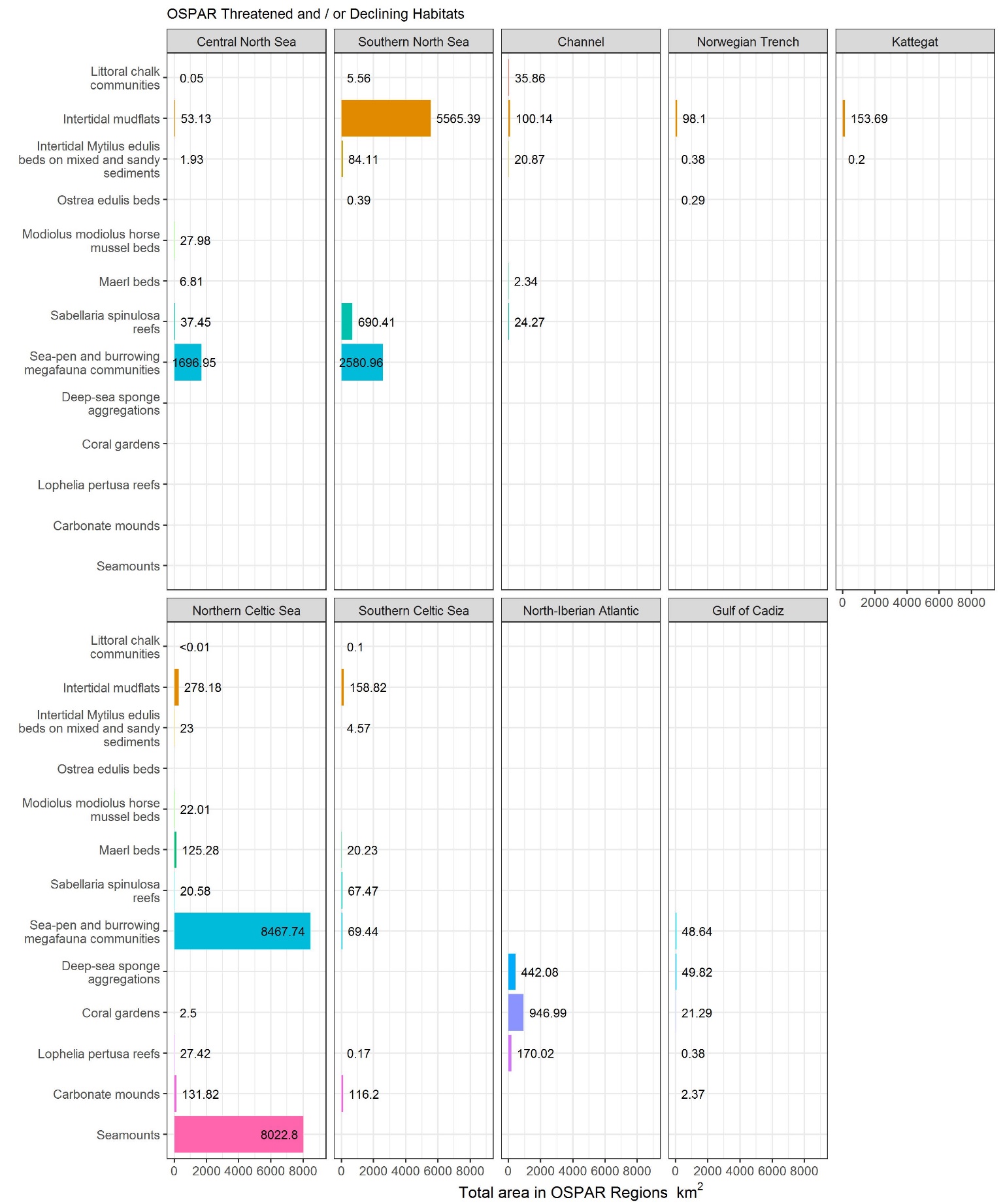
Figure bt: Total area (km2) of OSPAR Threatened and / or Declining habitats in Common Indicator Assessment Units (note: assessment units without reported data are not included; Atlantic projection, Faroe Shetland Waters, Gulf of Biscay, and South Iberian Atlantic)
Comparisons with previous assessments
The previous BH3 assessment (OSPAR Commission, 2017a) reported disturbance results for the assessment period 2010 to 2015 in Regions II and III (disturbance was also mapped in Region IV but results were not analysed due to data limitations). The current BH3 assessments used improved and updated data layers and updated methods, especially for sensitivity assessments; changes to the assessment units; and use of an overlapping assessment period, which included the IA 2017 timeframe (2009 to 2020). Subsequently, a direct comparison with the previous BH3 assessment (OSPAR Commission, 2017a) was not possible, due to the aforementioned caveats and interpretations of differences were mostly likely attributed to the newly improved EUNIS Level 4, 5 and 6 habitat and sensitivity data that were previously assessed at EUNIS Level 3 only. This was most apparent in the changes observed in disturbance in the Channel. Disturbance in the Channel in the QSR 2023 was considerably lower than that observed in the OSPAR Intermediate Assessment, 2017. The reduction was the direct result of improved resolution of detail in sensitivity and habitat data, facilitating biotope-resolution assessments (e.g., where only broadscale assessments were previously feasible).
Confidence assessments
The confidence of input habitat and sensitivity data were assessed using categorical scores (‘Low’, ‘Medium’, and ‘High’), based on the nature of the information, and combined to give an overall confidence score for abrasion sensitivity for each assessment period (Figure bu and Figure bv).

Figure bu: Confidence assessment of abrasion sensitivity across Common and Candidate Indicator Assessment Units in the 2009 to 2020 assessment period
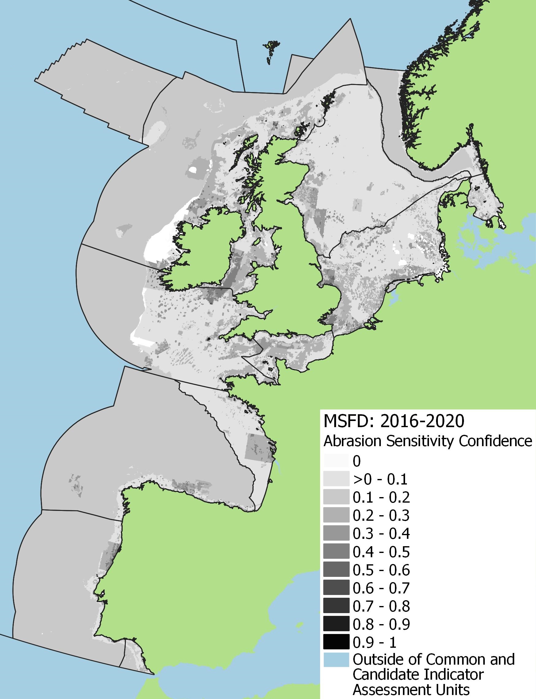
Figure bv: Confidence assessment of abrasion sensitivity across Common and Candidate Indicator Assessment Units in the 2016 to 2020 assessment period
Conclusion
This component of the BH3 QSR 2023 assessment evaluated benthic habitat disturbance in the North-East Atlantic associated with bottom-contact fishing over two timeframes (QSR:2009 to 2020; MSFD:2016 to 2020).
The assessment indicated a ubiquitous distribution of anthropogenic pressure across the OSPAR Maritime Area, where bottom-contact fishing was permitted to occur (< 800 m deep). All BHTs had ‘High’ and / or ‘Moderate’ disturbance, with Offshore circalittoral mud having the greatest proportion of ‘High’ disturbance and Offshore circalittoral coarse sediment recorded with the greatest proportion of ‘Low’ disturbance.
When considering the spatial distribution of disturbance, the greatest proportions of ‘High’ and ‘Moderate’ disturbance occurring together were in the Gulf of Biscay and the Southern North Sea, whereas the greatest proportion of ‘High’ disturbance alone was in the Gulf of Cadiz and the greatest proportion of ‘Low’ disturbance was in the Channel.
Disturbance was ‘Zero’ in approximately half of the area of Common Indicator Assessment Units in both QSR and MSFD assessments. However, gaps in the coverage of VMS data highlighted potential underestimations of disturbance in some areas and habitats. These aforementioned limitations associated with VMS data availability should be addressed in future assessments to facilitate more robust findings.
The BH3 QSR 2023 assessment evaluated physical disturbance to benthic habitats in the North-East Atlantic from bottom-contact fishing and commercial aggregate extraction; this component of the assessment is for fishing only. Analyses were conducted over two timeframes (where data were available), facilitating decadal OSPAR QSR and national reporting commitments for OSPAR Contracting Parties, (e.g., MSFD Article 8 assessments for Member States). Assessments were undertaken where BH3 is an agreed OSPAR Common Indicator: Regions II, III and IV, and where BH3 is an OSPAR Candidate Indicator: Region V. The method has been developed, tested, and critically reviewed by national experts from Contracting Parties within the OSPAR framework to ensure scientific integrity and representativity of findings.
In the QSR assessment, 13% of the total assessed area had ‘High’ disturbance and 23% had ‘Moderate’ disturbance, whilst in the MSFD assessment these proportions were 11% and 19%, respectively. In both assessments, 18% of the assessed area had ‘Low’ disturbance and 45% and 50% had ‘Zero’ disturbance in the QSR and MSFD assessments respectively. The distribution of disturbance was ubiquitous across the OSPAR Maritime Area, where bottom-contacting fishing was permitted to occur (<800 m deep). All BHTs had ‘High’ and/or ‘Moderate’ disturbance throughout both assessment periods, with Offshore circalittoral mud recorded as having the greatest proportion of ‘High’ disturbance. Conversely, Offshore circalittoral coarse sediment was found to have the greatest proportion of ‘Low’ disturbance. ‘High’ disturbance resulted from sensitive habitats, with species less tolerant or susceptible to impact, coinciding with high levels of pressure.
When considering the spatial distribution of disturbance in both assessment periods, the greatest proportions of ‘High’ and ‘Moderate’ disturbance occurring together were in the Gulf of Biscay and the Southern North Sea, whereas the greatest proportion of ‘High’ disturbance alone was in the Gulf of Cadiz. ‘High’ disturbance in the Gulf of Cadiz assessments was influenced both by the presence of sensitive habitats such as Offshore circalittoral mud and by peaks in observed ‘High’ disturbance in 2018 and 2020. In contrast, the greatest percentage of area with ‘Low’ disturbance was recorded in the Channel, which also had the greatest proportion of consistently ‘Low’ annual disturbance throughout both assessment periods. Disturbance in the Channel was considerably lower than observed in the OSPAR Intermediate Assessment, 2017, and is likely to be the direct result of improved resolution of detail in sensitivity and habitat data, facilitating biotope-resolution assessments (e.g., EUNIS Level 4) where only broadscale (e.g., EUNIS Level 3) assessments were previously feasible.
Habitats within United Kingdom MPAs were found to have higher disturbance than surrounding areas with similar levels of pressure, and were therefore, easily identified in mapped outputs. Although MPAs will generally have habitats determined from in-situ survey data, and therefore higher confidence than surrounding modelled data, protected features were designated and mapped at EUNIS Level 3. Following the precautionary approach of assessing sensitivity using assessments from child biotopes, these EUNIS Level 3 habitats were more likely to have higher assessed sensitivity and therefore, higher disturbance than adjacent areas of similar habitats mapped at EUNIS Level 4 and above. Habitat maps within United Kingdom MPAs were only available at EUNIS Level 3 (the scale of feature designation), resulting in MPA boundary outlines being clearly visible when disturbance was calculated (due to higher EUNIS Level 3-scale sensitivities).
It should be noted that disturbance occurred in 53% of the area of Common Indicator assessment units in the QSR period and in 48% in the MSFD assessment, where pressure and sensitivity data, alongside suitable habitat maps were jointly available. Disturbance could not be calculated in 2% of the area of Common Indicator assessment units where habitat or sensitivity data was incomplete. Furthermore, VMS data were absent in almost half of the assessed area in both assessments, although categorised as ‘Zero’ disturbance, some areas of data paucity remained.
Assessed disturbance was derived from interactions between sensitivity and pressure, and was therefore, dependent on sensitivity information being available and at relevant spatiotemporal scales. Data representative of unimpacted habitats or pristine reference conditions were not available, therefore habitat maps that represented an already impacted state may have been used to map sensitivity. However, it should be noted that following consultation and review by experts within the OSPAR framework, the BH3 method was improved in the QSR assessment, adapting how species records were analysed in order to mitigate erroneously mapping sensitivity with records from resilient species, in less resilient areas.
Sensitivity information at the time of assessment was most relevant to waters in northern Europe (e.g., United Kingdom, France, Germany); sensitivity information was not available from all biogeographic areas of the OSPAR Maritime Area. Future assessments will include locally-specific, improved sensitivity data, where available, and explore integration with other OSPAR indicators to ground-truth results in areas of knowledge gaps, such as the Gulf of Biscay, North- and South-Iberian Atlantic and Gulf of Cadiz. Findings in the QSR assessments were reviewed and critiqued by national experts, maximising regionally-specific accuracy with the data available. Furthermore, due to limitations associated with available activity data (e.g., missing fleets and vessels < 12 m) receptor recovery in the absence of pressure could not be assessed at the time of this assessment and will be explored further in future work.
The BH3 Indicator Assessment used in-situ survey data, where available. However, due to limited coverage of survey datasets, modelled habitat data were used to create a habitat map at an OSPAR-scale resolution. Furthermore, due to limitations associated with OSPAR Threatened and / or Declining Habitats GIS data, it was possible that some analysed features (in particular, historic, and uncertain records) were no longer present or had changed in extent during the assessment period. In addition, certain threatened and / or declining habitats may have been underreported in areas where habitat mapping data was scarce and / or limited in resolution (e.g., deep-sea areas).
The assessments of Threatened and / or Declining Habitats indicated that Sea-pen and burrowing megafauna communities was the habitat with highest disturbance. In the 2009 to 2020 assessment period, physical disturbance occurred in 98% of the total area of Sea-pen and burrowing megafauna communities across all Common Indicator Assessment Units where the feature was reported.
The assessment of disturbance to seafloor habitats from bottom-contacting fishing was constrained to the resolution and confidence of available VMS data. The aggregation of fishing vessel data to c-squares limited the confidence of disturbance impacts at a greater resolution when potential impacts may have been more locally focused. To some extent, the overlap of fishing pressure represented at c-square resolution with habitats unsuitable for bottom-contacting gear was highlighted by the presence of ‘Unassessed Disturbance’ in ‘rock and biogenic reef’ BHTs. Sensitivity in habitats not suitable for fishing were often unassessed or considered not relevant to the pressure and therefore, could not be assessed for disturbance. Additionally, the ‘rock and biogenic reef’ BHTs also include biogenic reefs on sediment habitats, for example ‘A5.61 Sublittoral polychaete worm reefs on sediment’. Some of these biogenic reef habitats are at risk of disturbance from bottom-contacting fishing and their aggregation to BHTs with other component habitats unsuitable for fishing could have resulted in a misrepresentation of disturbance in biogenic reef habitats.
Not all fleets fishing in the OSPAR Maritime Area were included in the assessments and were therefore, not accounted for in the results. Without more complete fishing pressure data it was not possible to make a high-confidence assessment of areas without risk of physical disturbance from these pressures. Furthermore, disturbance results should be treated with caution and are likely to be under-reported in areas where fleets not included in the VMS data are likely to have operated.
Confidence
Improvement to the BH3 indicator is a cyclical, iterative process, with continuous development via participatory engagement in OSPAR, ensuring that data and methods used are robust and utilise best available evidence and technologies. Algorithms and calculations will be adapted in the future, and where required, calibrated to improve integration with other OSPAR indicators to maximise confidence and accuracy of results. BH3 currently assesses physical disturbance associated with bottom-contact fishing and commercial aggregate extraction; new human activities will be considered in future assessments, where agreed and data are available.
Knowledge Gaps
In the QSR 2023 assessment, key areas of data deficiency and knowledge gaps were highlighted, including a lack of and restricted access to commercially sensitive pressure data. Habitat information was not available in all areas where pressure was reported, and an agreed OSPAR-scale habitat classification was not available. The limited availability of reference condition habitat data and pressure-state relationships at the regional scale resulted in reliance on expert knowledge and extrapolation of available pressure-state data. Integration with other benthic habitat indicators was not possible in the assessment and will require further testing when sufficient data is available.
Habitat data
The BH3 Indicator Assessment used the best available in-situ habitat data incorporated into the OSPAR-scale composite habitat map. However, the use of in-situ data at the scale of Common and Candidate Indicator Assessment Units alone was not feasible due to data paucity and modelled habitat maps were required to supplement in-situ data. Despite the combined use of modelled and in-situ data, habitat information was still not available for some locations, such as to the west of Ireland, limiting the total area that could be assessed for disturbance. There also remained areas where high-resolution habitat data were not publicly available, such as the Kattegat, due to data usage constraints and data confidentiality. In addition, the OSPAR Threatened and / or Declining Habitats GIS layer comprised data submitted by OSPAR Contracting Parties via data calls, which potentially included habitats with historic extents that may have changed during assessment periods, reducing their associated confidence. Furthermore, it was possible that in areas of data paucity, habitat extent may have been underreported in areas such as the deep sea.
Increased coverage of current, representative in-situ habitat data from surveys would improve confidence in results and increase the overall accuracy of maps via reduced reliance on models and by ground-truthing interpolated data. In addition, the incorporation of industry data into habitat maps, and additional survey work of benthic habitats (e.g., via improved Benthic Monitoring Programmes in areas outside of MPAs), would help increase data coverage. In addition to improved data availability, standardised habitat classifications, with accurate translations to wider classification systems are of paramount importance to facilitate integrated assessments across the OSPAR Maritime Area. The QSR 2023 assessment delivered disturbance assessments in EUNIS 2007, with results presented in MSFD BHT classifications to support Article 8 reporting of the EU Marine Strategy Framework Directive (MSFD). However, to further future assessments, additional work is required to better facilitate successful translations between commonly used habitat classifications (e.g., EUNIS 2007 and EUNIS 2019), to ensure OSPAR benthic indicator interoperability (see further details in the QSR 2023 BH4 report section ‘Knowledge Gaps’).
Sensitivity data
A key knowledge gap identified in this assessment included the absence of sensitivity information for certain MSFD BHTs and Other Habitat Types (OHTs), the latter including the OSPAR T&D habitats and species, particularly in areas such as the deep sea. More complete data on seafloor sensitivity to pressure and knowledge of activity-pressure-receptor relationships can be acquired through improved understanding of the resistance and resilience of species and habitats, alongside additional research at relevant spatiotemporal scales (e.g., EUNIS Levels 4, 5 and 6). The QSR 2023 BH3 assessment enabled detailed biotope-resolution sensitivity and disturbance assessments, which improved the accuracy of outputs when compared with the IA 2017. However, in the absence of direct sensitivity assessments, the aggregation of sensitivity from EUNIS levels 4 to 6 to levels 2 to 3, and the translations between EUNIS and MSFD classifications may have resulted in both an over and underestimation of the sensitivity of individual BHT polygons. Therefore, habitat-specific sensitivity scores require further testing and validation to help improve application to future assessments.
In addition, the mapping of sensitivity could be improved through the availability of a consistent OSPAR-scale habitat classification system (including versions, e.g., EUNIS 2007, 2019, 2022) and the availability of methods to translate between habitat classifications accurately. This would enable Contracting Parties to ensure the interoperability of sensitivity data to facilitate integrated assessments at a North-East Atlantic scale. At the time of assessment, translations between EUNIS 2007 and EUNIS 2019 were not possible due to errors in available translation tables. Work was undertaken through EMODnet and the European Environment Agency to address the identified errors, although, outputs were not available in the required timeframes for the delivery of the QSR 2023. Therefore, this assessment used EUNIS 2007 only, and translated to MSFD BHT via biological zone data available via EMODnet.
Furthermore, sensitivity information available at the time of the assessment was most relevant to areas with a similar biogeography to the waters surrounding the United Kingdom, and therefore, would be improved with sensitivity assessments from all biogeographic areas of the OSPAR Maritime Area. Integration with other benthic indicators such as the Sentinels of Seabed (SoS) indicator (BH1) (Serrano et al., 2022) and Condition of Benthic Habitat Communities (BH2) (OSPAR, 2018) into the BH3 method will further broaden the evidence base used in assessments in biogeographic regions and will be explored in future work.
In the QSR assessment, the BH3 method was improved by experts collaborating through the OSPAR framework to account for resilient species present in less resilient habitats. However, understanding of ecosystem change in response to pressure could be furthered through the availability of data from unimpacted species and habitats to serve as reference when assessing sensitivity. Moreover, data where fishing pressure has been removed (e.g., no-take zones) would help improve understanding of receptor recovery and will be explored in future work (please note, improved VMS data for missing fleets and vessels < 12 m would be beneficial).
Pressure data
The BH3 assessment of the risk of physical disturbance from human activities only assessed three pressures associated with human activities. Two of these pressures, surface and subsurface abrasion from bottom-contact fisheries, were detailed in this assessment; see the separate BH3b assessment for risk of disturbance from extraction pressure from commercial aggregate extraction activities. New human activities will be considered in future assessments, where agreed and data are available. Therefore, the BH3 indicator will be further developed to support further implementation as an indicator of physical disturbance of the seabed, and future assessments of the risk of adverse anthropogenic effects.
Due to data paucity in available VMS information, the spatial extent of pressures associated with bottom-contact fishing activity could have been underestimated in some areas. In inshore areas, the future inclusion of Inshore Vessel Monitoring Systems (I-VMS) data in assessments would increase the confidence of assessments in inshore waters, where smaller vessels are most likely to operate. Additionally, VMS data from Portugal and Norway were not included in the assessment, as the data did not pass ICES quality assurance checks or, in the case of Iceland, was not submitted. Therefore, bottom-contact fishing pressure may have appeared to be absent and / or underrepresented, despite fleet activities having taken place. The improvement of VMS data quality assurance protocols by OSPAR Contracting Parties prior to submission of data to ICES will improve the coverage of pressure data in future assessments. Furthermore, VMS data obtained from ICES via the OSPAR data call did not cover the entirety of Kattegat (areas around Ise Fjord and Roskilde Fjord). The new OSPAR benthic habitat assessment units extended beyond the original spatial extent of the official OSPAR Region boundaries used in the data call, which resulted in the potential absence of VMS data. In future assessments, modifications to assessment units that potentially extend beyond the areas agreed in the data call could results in similar knowledge gaps and should be accounted for, where feasible.
Conversely, there were also areas where there was high confidence that the extent of bottom-contact fishing activity had been overestimated. Due to limitations associated with how fishing intensity was calculated from VMS data, activity may have been overestimated in areas where vessel speeds were likely to be reduced during transit near ports or in adverse weather conditions and were inaccurately attributed to speeds associated with trawling activity. Where erroneous VMS data were highlighted by national experts, disturbance methods were adapted to remove misleading results (e.g., Swedish No Trawl Zone and deep-sea areas of the Northern-Iberian Atlantic). Furthermore, although the best available data for the physical pressure of bottom-contacting fishing gears on the seabed was used at the time of assessment, knowledge gaps were identified regarding the distribution and intensity of pressure within individual c-squares. The confidence in the spatial distribution of categorical values of fishing pressure could potentially be improved using alternative estimates that address limitations inherent with estimated vessel tracks from 2-hour ping intervals, arbitrary grid-cell size, and the assumption that pressure and intensity are homogeneous in distribution within grid cells (Gerritsen, Minto and Lordan, 2013).
The BH3 assessment of the risk of disturbance from physical abrasion pressures associated with bottom-contact fisheries categorised and assessed surface and subsurface Swept Area Ratios (SAR) separately, following the agreed method used previously in the Intermediate Assessment (OSPAR, 2017a). Future work investigating the response of benthic habitats to consistent or variable abrasion pressure would help inform how pressure impacts could be best represented across an assessment period.
Disturbance results
Knowledge gaps remain in the current understanding of biological responses to adverse effects caused by fishing pressure, and other pressures associated with physical disturbance. Calibration with the results of other benthic indicators such as the Sentinels of Seabed (SoS) indicator (BH1) (Serrano et al., 2022) and validation with indicators such as Condition of Benthic Habitat Communities (BH2b) (OSPAR, 2018) will be explored in future work. Furthermore, where improved datasets become available, data-based assessments of the effects physical pressures have on benthic faunal and floral receptors will be explored in future work to mitigate aforementioned limitations that can affect the certainty and accuracy of indicator outputs.
Geographical application
At present BH3 is still being investigated for its application in Arctic Waters and the Wider Atlantic, mainly due to limited data availability within these Regions. It is anticipated that data on habitat distribution and sensitivity will be included at a later stage, to allow the analysis to address the wider spatial scale and assess variations in disturbance across OSPAR regions more accurately.
BioConsult, 2013. Seafloor integrity - Physical damage, having regard to substrate characteristics (Descriptor 6). A conceptual approach for the assessment of indicator 6.1.2: ‘Extent of the seafloor significantly affected by human activities for the different substrate types’. Report within the R & D project ‘Compilation and assessment of selected anthropogenic pressures in the context of the Marine Strategy Framework Directive’, UFOPLAN 3710 25 206.
Castle L., Lillis H., Duncan G. & Manca E., 2021. Method for creating a EUNIS level 3 seabed habitat map integrating fine- and broad-scale maps for the North-East Atlantic. JNCC report in Prep.
Church N.J., Carter A.J., Tobin D., Edwards D., Eassom A., Cameron A., Johnson G.E., Robson, L.M. & Webb K.E., 2016. JNCC Recommended Pressure Mapping Methodology 1. Abrasion: Methods paper for creating a geo-data layer for the pressure ‘Physical Damage (Reversible Change) - Penetration and / or disturbance of the substrate below the surface of the seabed, including abrasion’. JNCC report No. 515, JNCC, Peterborough.
Collie, J. S., Hall., S. J., Kaiser, M. J., and Poiner, I. R. 2001. A quantitative analysis of fishing impacts on shelf-sea benthos. Journal of Animal Ecology, 69(5); 7785-798
Defra, 2015. Validating an Activity-Pressure Matrix. Report R.2435.
Deporte, N., Ulrich, C., Mahévas, S., Demanèche, S., Bastardie, F., 2012. Regional métier definition: a comparative investigation of statistical methods using a workflow applied to international otter trawl fisheries in the North Sea. ICES Journal of Marine Science, Volume 69, Issue 2, March 2012, Pages 331–342.
Eigaard, O.R., Bastardie, F., Breen, M., Dinesen, G.E., Hintzen, N.T., Laffargue, P., Mortensen, L.O., Rasmus Nielsen, J., Nilsson, H.C., O’Neill, F.G., Polet, H., Reid, D.G., Sala, A., Sköld, M., Smith, C., Sørensen, T.K., Tully, O., Zengin, M., Rijnsdorp A.D., 2016. Estimating seabed pressure from demersal trawls, seines, and dredges based on gear design and dimensions. ICES Journal of Marine Science, Volume 73, Issue suppl_1, January 2016, Pages i27–i43.
Ellwood, H. 2014. Creating a EUNIS level 3 seabed habitat map integrating data originating from maps from field surveys and the EUSeaMap model. JNCC 2010 MESH Confidence Assessment. [Online] Available at: http://www.emodnet-seabedhabitats.eu/default.aspx?page=1635 (Accessed: 01/12/2021).
EMODnet, 2020. OSPAR Habitats in the North-East Atlantic Ocean - 2020 Polygons [Online] Available at: http://www.emodnet-seabedhabitats.eu/access-data/download-data/?linkid=ospar_2020_poly (Accessed: 01/12/2021).
EMODnet, 2021. Seabed Habitats. [Online] Available at: https://emodnet.ec.europa.eu/en/seabed-habitats (Accessed: 01/12/2021).
EMODnet Bathymetry Consortium. 2020. EMODnet Digital Bathymetry (DTM). Available at: https://portal.emodnet-bathymetry.eu/?menu=19 (Accessed 09/08/2022).
Eno, N.C., Frid, C. L. J., Hall, K., Ramsay, K., Sharp, R. A. M., Brazier, D. P., Hearn, S., Dernie, K. M., Robinson, K. A, Paramor, O. A. L., and Robinson, L. A. 2013. Assessing the sensitivity of habitats to fishing: from seabed maps to sensitivity maps. Journal of Fish Biology, 83, 826-846
ESRI, 2012. ArcGIS Release 10.1. Redlands, CA.
European Environment Agency, (EEA), 2017. EEA marine assessment grid, Jan. 2017. European Environment Agency Geospatial Data Catalogue. [Online] Available at: https://sdi.eea.europa.eu/catalogue/srv/eng/catalog.search#/metadata/84d1f816-1913-45b1-94b7-a5721a18296c (Accessed 08/11/2021).
European Environment Agency, (EEA), 2021. EUNIS Habitat Classification. [Online] Available at: https://eunis.eea.europa.eu/habitats-code-browser-revised.jsp (Accessed: 08/11/2021).
Garrard, S.M., Perry, F. & Tyler-Walters, H., 2019. Discrete Lophelia pertusa colonies on Atlantic mid bathyal rock and other hard substrata. In Tyler-Walters H. and Hiscock K. Marine Life Information Network: Biology and Sensitivity Key Information Reviews, Plymouth Marine Biological Association of the United Kingdom.
Garrard, S.M., Perry, F. & Tyler-Walters, H., 2020. Discrete Lophelia pertusa colonies on Atlantic upper bathyal rock and other hard substrata. In Tyler-Walters H. and Hiscock K. Marine Life Information Network: Biology and Sensitivity Key Information Reviews, Plymouth Marine Biological Association of the United Kingdom.
Gerritsen, H., Minto, C. and Lordan, C., 2013. How much of the seabed is impacted by mobile fishing gear? Absolute estimates from Vessel Monitoring System (VMS) point data. ICES Journal of Marine Science, 70(3), pp.523-531.
Holling C.S., 1973. Resilience and stability of ecological systems. Annual Review of Ecology and Systematics, 4(1), 1-23.
ICES, 2015. Report of the Working Group on Spatial Fisheries Data (WGSFD).
ICES, 2021. OSPAR request on the production of spatial data layers of fishing intensity / pressure. ICES Technical service.
JNCC, 2011. Review of methods for mapping anthropogenic pressures in UK waters in support of the Marine Biodiversity Monitoring R&D Programme. Briefing paper to UKMMAS evidence groups. Presented 06/10/2011.
Lambert, G. I., Jennings, S., Kaiser, M. J., Davies, T. W., and Hiddink, J. G., 2014. Quantifying recovery rates and resilience of seabed habitats impacted by bottom fishing. Journal of Applied Ecology, 51(5); 1326-1336.
Last, E.K., Matear, L. & Robson, L.M., 2020. Developing a method for broadscale & feature-level sensitivity assessments: the MarESA aggregation. JNCC Report No. 662, JNCC, Peterborough, ISSN 0963-8091.
Last, E.K., Ferguson, M. & Robson, L.M. 2019a. Mixed coral assemblage on Atlantic mid bathyal Lophelia pertusa reef framework (biogenic structure). In Tyler-Walters H. Marine Life Information Network: Biology and Sensitivity Key Information Reviews. Plymouth Marine Biological Association of the United Kingdom.
Last, E.K., Ferguson, M. & Robson, L.M. 2019b. Mixed coral assemblage on Atlantic upper bathyal Lophelia pertusa reef framework (biogenic structure). In Tyler-Walters H. Marine Life Information Network: Biology and Sensitivity Key Information Reviews. Plymouth Marine Biological Association of the United Kingdom.
Maher, E. & Alexander, D., 2016. Marine Rocky Habitat Ecological Groups and their Sensitivity to Pressures Associated with Human Activities, JNCC Report 589A.
Maher, E., Cramb, P., de Ros Moliner, A., Alexander, D. & Rengstorf, A., (2016), Assessing the sensitivity of sublittoral rock habitats to pressures associated with marine activities, JNCC Report No. 589B, JNCC, Peterborough, ISSN 0963-8091.
Manca, E. and Lillis H., 2022. 2019 Update to UKSeaMap – a broad-scale seabed habitat map for the UK. Unpublished.
Moss, D., 2008. EUNIS Habitat classification - a guide for users. European Topic Centre on Biological Diversity. [Online] Available at: https://www.eea.europa.eu/data-and-maps/data/eunis-habitat-classification (Accessed 03/02/2022)
McQuatters-Gollop, A.., Guerin, L., Arroyo, N.L., Aubert, A., Artigas, L.F, Bedford, J., Corcoran, E., Dierschke, V., Elliott, S.A.M., Geelhoed, S.C.V., Gilles, A., Gonzalez-Irusta, J.M., Haelters, J., Johansen, M., Le Loc’h, F., Lynam, C.P., Niquil, N., Meakins, B., Mitchell, I., Padegimas, B., Pesch, R., Preciado, I., Rombouts, I., Safi, G., Schmitt, P., Schückel, U., Serrano, A., Stebbing, P., De la Torriente, & A., Vina-Herbon, C., 2022. Assessing the state of marine biodiversity in the Northeast Atlantic. Ecological Indicators, 141, 109148.
OSPAR Commission, 2008. OSPAR List of Threatened and / or Declining Species and Habitats (OSPAR Agreement 2008-06) [Online] Available at: https://www.ospar.org/documents?d=32794
OSPAR Commission, 2011. Pressure list and descriptions. Paper to ICG-COBAM 11/8/1 Add.1-E (amended version 25th March 2011) presented by ICG-Cumulative Effects. OSPAR Commission, London.
OSPAR Commission, 2014. OSPAR Joint Assessment and Monitoring Programme (JAMP) 2014-2023.
OSPAR Commission, 2017a. OSPAR Intermediate Assessment 2017. OSPAR Commission. London.
OSPAR Commission, 2017b. OSPAR Coordinated Environmental Monitoring Programme (CEMP) Guidelines. Common Indicator: BH3 Extent of Physical damage to predominant and special habitats (https://www.ospar.org/documents?v=37641).
OSPAR Commission, 2018. OSPAR Coordinated Environmental Monitoring Programme (CEMP) Guidelines- 2023 update. Common indicator: Condition of benthic habitat communities (BH2) – common approach (https://www.ospar.org/documents?v=39000)
OSPAR Commission, 2019. QSR 2023 Guidance Document. OSPAR Agreement 2019-02.
OSPAR Commission, 2022. List of Threatened and / or Declining Species & Habitats; Habitats [Online] Available at: https://www.ospar.org/work-areas/bdc/species-habitats/list-of-threatened-declining-species-habitats/habitats (Accessed 01/02/2022)
Python Software Foundation, 2020. Python Language Reference, version 3.7.11.
R Core Team, 2019. R: A language and environment for statistical computing. R Foundation for Statistical Computing, Vienna, Austria.
R Core Team, 2020. R: A language and environment for statistical computing. R Foundation for Statistical Computing, Vienna, Austria.
R Core Team, 2021. R: A language and environment for statistical computing. R Foundation for Statistical Computing, Vienna, Austria.
Robinson, L.A., Rogers S. & Frid, C.L.J., 2008. A marine assessment and monitoring framework for application by UKMMAS and OSPAR - Assessment of Pressures and Impacts. Phase II: Application for regional assessments. JNCC Contract No: C-08-0007-0027. UKMMAS, 2010. Charting Progress 2.
Robson, L.M., Fincham, J., Peckett, F.J., Frost, N., Jackson, C., Carter, A.J. & Matear, L. 2018. UK Marine Pressures-Activities Database “PAD”: Methods Report. JNCC Report No. 624, JNCC, Peterborough, ISSN 0963-8091.
Rondinini, C. 2010. Meeting the MPA network design principles of representation and adequacy: developing species-area curves for habitats. JNCC Report No. 439. JNCC, Peterborough
Sanders, M. J., and Morgan, A. J., 1976. Fishing power, fishing effort, density, fishing intensity and fishing mortality. ICES Journal of Marine Sciences, 37(1), 36-40.
Schroeder, A., Gutow, L., & Gusky, M., 2008. FishPact. Auswirkungen von Grundschleppnetzfischereien sowie von Sand- und Kiesabbauvorhaben auf die Meeresbodenstruktur und das Benthos in den Schutzgebieten der deutschen AWZ der Nordsee (MAR 36032/15). Report for the Bundesamt für Naturschutz.
Serrano, A., de la Torrientea A., Punzóna, A., Blancoa, M., Bellas, J., Durán-Muñoz, P., Murillo, F.J., Sacau, M., García-Alegrea, A., Antolíneza, A., Elliott, S., Guerine, L., Vina-Herbón, C.V., Marra, S., González-Irustaa, J.M., 2022. Sentinels of Seabed (SoS) indicator: Assessing benthic habitats condition using typical and sensitive species. Ecological Indicators, 140, 108979.
Tillin, H.M., Hull, S.C. & Tyler-Walters, H., 2010. Development of a Sensitivity Matrix (pressures-MCZ / MPA features). Defra Contract No. MB0102 Task 3A, Report No. 22.
Tillin, H., Tyler-Walters, H., 2014a. Assessing the sensitivity of subtidal sedimentary habitats to pressures associated with marine activities. Phase 1 Report: Rationale and proposed ecological groupings for Level 5 biotopes against which sensitivity assessments would be best undertaken. JNCC Report No. 512A, 68 pp.
Tillin, H. & Tyler-Walters, H., 2014b. Assessing the sensitivity of subtidal sedimentary habitats to pressures associated with marine activities. Phase 2 Report – Literature review and sensitivity assessments for ecological groups for circalittoral and offshore Level 5 biotopes. JNCC Report No. 512B, 260 pp.
Tillin, H.M. & Tyler-Walters, H., 2015. Finalised list of definitions of pressures and benchmarks for sensitivity assessment. 7-9.
Tyler-Walters, H., Tillin, H.M., d’Avack, E.A.S., Perry, F. & Stamp, T., 2018. Marine Evidence based Sensitivity Assessment (MarESA) – A Guide. Plymouth: Marine Biological Association.
Van Denderen, P. D., Bolam, S. G., Hiddink, J. G., Jennings, S., Kenny, A., Rijnsdorp, A. D., and van Kooten, T., 2015. Similar effects of bottom trawling an natural disturbance on composition and function of benthic communities across habitats. Marine Ecology Progress Series, 341, 31-43.
Van Loon, W.M.G.M., Walvoort, D.J., Van Hoey, G., Vina-Herbon, C., Blandon, A., Pesch, R., Schmitt, P., Scholle, J., Heyer, K., Lavaleye, M. and Phillips, G., 2018. A regional benthic fauna assessment method for the Southern North Sea using Margalef diversity and reference value modelling. Ecological Indicators, 89, 667-679.
Vasquez, M., Allen, H., Manca, E., Castle, L., Lillis, H., Agnesi, S., Al Hamdani, Z., Annunziatellis, A., Askew, N., Bekkby, T., Bentes, L., Doncheva, V., Drakopoulou, V., Duncan, G., Gonçalves, J., Inghilesi, R., Laamanen, L., Loukaidi, V., Martin, S., McGrath, F., Mo, G., Monteiro, P., Muresan, M., Nikilova, C., O'Keeffe, E., Pesch, R., Pinder, J., Populus, J., Ridgeway, A., Sakellariou, D., Teaca, A., Tempera, F., Todorova, V., Tunesi, L. & Virtanen, E., 2021. EUSeaMap 2021, A European broad-scale seabed habitat map, Technical Report.
Contributors
Lead Authors: Liam Matear and Cristina Vina-Herbon
Supporting Authors: Kirsty Woodcock, Stephen Duncombe-Smith, Adam Smith, Petra Schmitt, Axel Kreutle, Stefano Marra, Emma Curtis, Holly Baigent
Supported by: OSPAR Benthic Habitat Expert Group (OBHEG), Intersessional Correspondence Group on the Coordination of Biodiversity Assessment and Monitoring (ICG-COBAM), OSPAR Biodiversity Committee (BDC)
Delivered by
This work was co-funded by the European Maritime and Fisheries Fund through the project: “North-east Atlantic project on biodiversity and eutrophication assessment integration and creation of effective measures (NEA PANACEA)”, financed by the European Union’s DG ENV/MSFD 2020, under agreement No. 110661/2020/839628/SUB/ENV.C.2.
 |  |
Citation
Matear, L., Vina-Herbon, C., Woodcock, K.A., Duncombe-Smith, S.W., Smith, A.P., Schmitt, P., Kreutle, A., Marra, S., Curtis, E.J., and Baigent, H.N. 2023. Extent of Physical Disturbance to Benthic Habitats: Fisheries. In: OSPAR, 2023: The 2023 Quality Status Report for the Northeast Atlantic. OSPAR Commission, London. Available at: https://oap.ospar.org/en/ospar-assessments/quality-status-reports/qsr-2023/indicator-assessments/phys-dist-habs-fisheries/
| Assessment type | Indicator Assessment |
|---|---|
| Summary Results | https://odims.ospar.org/en/submissions/ospar_ospar_phy_disturb_fis_msfd_2023_06/ |
| SDG Indicator | 14.2 By 2020, sustainably manage and protect marine and coastal ecosystems to avoid significant adverse impacts, including by strengthening their resilience, and take action for their restoration in order to achieve healthy and productive oceans |
| Thematic Activity | Biological Diversity and Ecosystems |
| Relevant OSPAR Documentation | OSPAR Agreement 2008-06 List of Threatened and / or Declining Species and Habitats |
| Linkage | https://www.ospar.org/work-areas/bdc/species-habitats/list-of-threatened-declining-species-habitats/habitats |
| Date of publication | 2023-06-30 |
| Conditions applying to access and use | https://oap.ospar.org/en/data-policy/ |
| Data Results | . |
| Data Snapshot | https://odims.ospar.org/en/submissions/ospar_phys_dist_habs_dsnap_2023_06/ |