

Effect of underwater noise on the state of the marine environment
Effect of continuous noise on state of marine environment
The material in this section is taken from OSPAR’s Candidate Indicator on Pressure from Ambient Noise , where more detailed information on the indicator methodology is presented.
The thresholds at which continuous noise from human activities is of concern is uncertain – for example, there is as yet no assessment of good environmental status for continuous noise under the Marine Strategy Framework Directive (2008/56/EC). Noise can affect marine animals through ‘masking’ – interfering with their ability to communicate, navigate, find food, or detect threats – or through behavioural disturbance, such as fleeing or distraction. The pressure index proposed in JOMOPANS specifically addresses masking, and is set at an excess level of 20 dB or more above natural background levels. This gives a clear discrimination in the ‘dominance map’ below, but at this time there is no biological rationale behind the 20 dB level. Work on defining threshold values for continuous noise is in progress in OSPAR and in the EU.
Figure S.1 is a ‘dominance map’ which illustrates the percentage of time for which the ‘excess level’ is more than 20 dB for the 125 Hz band. The excess level is defined as the difference between total noise (from wind and ships) and the reference condition (i.e. natural background noise levels). In areas such as the Southern North Sea and the sea near the north-west of Denmark, shipping noise exceeds that threshold most of the time, whereas in some other areas (e.g. the Dogger Bank and the shallow parts of the Kattegat) sound pressure levels were within 20 dB of the reference condition for most of the time in the low frequency bands.

Figure S.1: Dominance map for a cut-off level of 20 dB of the excess level
Key message from indicator assessment
Shipping noise is dominant in the underwater soundscape of the North Sea. In the southern part and along the major shipping routes the noise exceeds the natural sound by more than 20 dB for more than 50% of the time.

Figure S.2: pressure curves for the 125 Hz band for continuous noise in the North Sea and for the MPAs within the North Sea
Exposure curves can be used to illustrate the extent to which geographical areas are subject to excess noise over time. They plot the percentage of a geographical area subject to noise above the excess level (20 dB) against the percentage of time with that excess. The area below the curve gives a pressure index, which can be compared between geographical areas. Figure S.2 below does this for various parts of the North Sea, and for marine protected areas (MPAs) within the North Sea. Some MPAs, many of which are in the southern part of the North Sea, are among the areas affected by particularly high levels of anthropogenic noise.
Effect of impulsive noise on the state of the marine environment
Impulsive sound can cause temporary displacement of cetaceans, physiological stress in fish, developmental abnormalities in invertebrate larvae and, in severe cases, permanent hearing damage and blast injuries. It remains uncertain what this means at the population or ecosystem scale and, as yet, there are no agreed threshold values for good environmental status for impulsive noise under the Marine Strategy Framework Directive.
The OSPAR Common Indicator on the Risk of Impact from Impulsive Noise addresses this by assessing the exposure to impulsive sound of species known to be particularly sensitive to disturbance or physiological stress from such sound. It analyses the distribution, in space and time, of impulsive sound sources and relates this to the distribution, again in space and time, of selected species or habitats. This produces an exposure assessment which is taken as a measure of the risk of impact on each species or habitat. A detailed explanation of the assessment methodology and information sources is given in the Common Indicator.
The first assessment under this Common Indicator uses the harbour porpoise as the indicator species. It is the most common cetacean in the North Sea, is particularly sensitive to impulsive sound, and has relatively high-quality modelled density estimates; as such, it is particularly suitable for this assessment and may serve as a sentinel for other cetaceans. Future assessments will consider additional species for risk assessment, and more comprehensive reporting in future years should reduce uncertainty in the impulsive sound activity used in the assessment.
Modelled densities of porpoise in the maritime area used for the assessment are shown in Figure S.3. Norwegian waters were not included because no impulsive noise data were available before 2019. The density data cover the months from March to November.
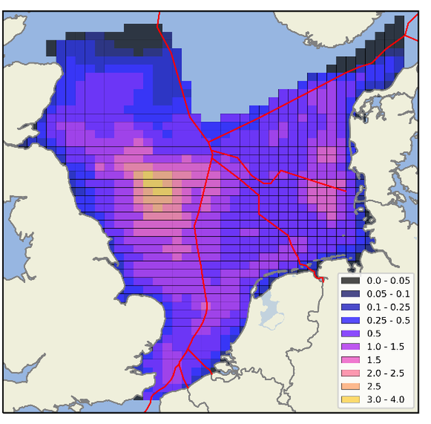
Figure S.3: Average annual density of harbour porpoise (animals per km2, March – November)
Combining information on harbour porpoise densities with information on sources of impulsive noise allows risk maps to be produced that show the extent to which pressure from impulsive noise coincides with the presence of porpoises. The metric used for the maps is the base 10 logarithm of the average number of pulse block days in each block across the assessment period (e.g. a month or year) multiplied by the number of animals estimated to be in that block at the time.
Risk map for harbour porpoise for 2015. Available at: ODIMS
Risk map for harbour porpoise for 2016. Available at: ODIMS
Risk map for harbour porpoise for 2017. Available at: ODIMS
Risk map for harbour porpoise for 2018. Available at: ODIMS
Risk map for harbour porpoise for 2019. Available at: ODIMS
Figure S.4: Annual risk maps for harbour porpoise for 2015-2019, March-November
Annual risk maps indicate that risk was more widespread in 2015 than in subsequent years, due to the large-scale seismic survey programme carried out by the United Kingdom Oil & Gas Authority at that time. Monthly risk maps can also be produced, which show that risk was most widespread from August - October.
Although data on harbour porpoise densities was not available for the winter months (December - February), estimates could be made for the extent of habitat area (Figure S.3) exposed to impulsive noise. For those months, the daily exposed habitat area was <2.5% in all years), while during March to October this was typically <5%.
In 2015 and 2016, most estimated disturbance resulted from seismic airguns, whereas in later years no single source dominated (see Table S.1 below). The low proportion estimated for piling in 2019 may be due to incomplete reporting. The indicator shows that highest noise exposure in 2017 and 2018 comes from piling, despite it being a relatively low contributor to pulse block days. This may be because populations of harbour porpoise tended to be in the areas favoured for offshore wind construction in those years.
| Source type | % of 2015 exposure | % of 2016 exposure | % of 2017 exposure | % of 2018 exposure | % of 2019 exposure |
|---|---|---|---|---|---|
| Explosions | 1 | 1 | 11 | 7 | 6 |
| Airgun array | 77 | 51 | 24 | 25 | 47 |
| Sonar/ADD | 0 | 0.1 | 0 | 0.2 | 0 |
| Generic | 2 | 23 | 19 | 35 | 37 |
| Piling | 16 | 22 | 42 | 31 | 2 |
| Multiple | 2 | 3 | 4 | 3 | 9 |
Key message from indicator assessment
The estimated risk of disturbance to harbour porpoise from reported anthropogenic impulsive sound decreased by 48% from 2015 to 2017, then increased by 31% from 2017 to 2019. Exposure of harbour porpoise to anthropogenic impulsive sound was typically greatest during August - October. More comprehensive reporting will improve confidence in the assessment.
The data can be used to produce exposure curves which plot the percentage of the porpoise population density exposed to impulsive noise against the percentage of the assessment period for which that exposure occurred. The area under the curve can be used to derive an exposure index (EI), a single number indicative of the overall amount of noise exposure for a population or habitat. The methodology used means that, for example, an exposure index of 20 is equivalent to 20% of the population or habitat being exposed for 20% of the assessment period.

Figure S.5: Annual exposure indices for harbour porpoise

Figure S.6: Corresponding exposure curves for harbour porpoise
More comprehensive reporting will improve confidence in the assessment. No overall trends in long-term noise levels can be inferred from these results.
The exposure curves show that a relatively small proportion of the population density was exposed for a large proportion of time (up to 95% of the assessment period during 2015). The majority of the population density was unexposed, with the maximum population in any one year exposed to any reported impulsive noise being approximately 13% in 2015. However, since the harbour porpoise is a highly mobile species, these results should not be interpreted as meaning that 13% of animals in the population were estimated to be exposed, but that 13% of the habitat was exposed when weighted for how frequently that habitat is used. The number of individual animals exposed may be much higher than 13% of the population, since individual animals may incur multiple exposures in different areas.
The effect of noise abatement systems used for pile driving operations in German, Danish, Dutch and Belgian waters was taken into account in the exposure indices. These were also modelled. They reduced the annual exposure indices, compared with unabated piling, by at least between 0.1 and 0.9, depending on the year. This is likely to be an underestimate in exposure reduction due to conservative assumptions underlying the exposure calculations.
Exposure in marine protected areas (MPAs) was also assessed. MPAs were not designated with noise management specifically in mind. The exposure index was lower inside the MPAs than outside during 2015, 2016 and 2019, but higher in the intervening years.
| Pressures | Impact |